Mapping SDGs Indicators

Get the data

The first step is to load the required libraries.

library(SDGsR)
library(tidyverse)
library(plotly)
library(shiny)

We are going to select Indicators from three Targets in Goal 15 “Life on land”. The Targets we are interested in are:

Target 15.6 “Promote fair and equitable sharing of the benefits arising from the utilization of genetic resources and promote appropriate access to such resources, as internationally agreed”;
Target 15.9 “By 2020, integrate ecosystem and biodiversity values into national and local planning, development processes, poverty reduction strategies and accounts”; and
Target 15.a.1 “Mobilize and significantly increase financial resources from all sources to conserve and sustainably use biodiversity and ecosystems”

The associated Indicators are:

15.6.1 “Number of countries that have adopted legislative, administrative and policy frameworks to ensure fair and equitable sharing of benefits”
15.9.1 “(a) Number of countries that have established national targets in accordance with or similar to Aichi Biodiversity Target 2 of the Strategic Plan for Biodiversity 2011–2020 in their national biodiversity strategy and action plans and the progress reported towards these targets; and (b) integration of biodiversity into national accounting and reporting systems, defined as implementation of the System of Environmental-Economic Accounting”
15.a.1 “Official development assistance on conservation and sustainable use of biodiversity; and (b) revenue generated and finance mobilized from biodiversity-relevant economic instruments”

There are several data series that are used to inform each Indicator (some may have one but others will have two or three different data series associated with them).

We can use the SDGSR::get_indicator_data() to connect to the SDGs API and download the data we need.

Ind_15.6.1<-get_indicator_data(indicator = '15.6.1')
Ind_15.9.1<-get_indicator_data(indicator = '15.9.1')
Ind_15.a.1<-get_indicator_data(indicator = '15.a.1')

Now we join the three datasets together and select the name of the country, the year, the Indicator value, the description of the series that the value relates to and the ISO three letter country code.

Ind_15.6.1<-Ind_15.6.1 %>% 
  group_by(seriesDescription, geoAreaName) %>% 
  select(geoAreaName, timePeriodStart,value, seriesDescription, geoAreaCode)
Ind_15.9.1<-Ind_15.9.1 %>% 
  group_by(seriesDescription, geoAreaName) %>% 
  select(geoAreaName, timePeriodStart,value, seriesDescription, geoAreaCode)
Ind_15.a.1<-Ind_15.a.1 %>% 
  group_by(seriesDescription, geoAreaName) %>% 
  select(geoAreaName, timePeriodStart,value, seriesDescription, geoAreaCode)
Ind_15_data=rbind(Ind_15.6.1,Ind_15.9.1, Ind_15.a.1)
Ind_15_data$Indicator=c(rep("Ind_15.6.1", dim(Ind_15.6.1)[1]), rep("Ind_15.9.1", dim(Ind_15.9.1)[1]), rep("Ind_15.a.1", dim(Ind_15.a.1)[1]))

Ind_15_data %>%
  head(4) %>% 
  kableExtra::kable()

geoAreaName	timePeriodStart	value	seriesDescription	geoAreaCode	Indicator
Afghanistan	2012	218	Total reported number of Standard Material Transfer Agreements (SMTAs) transferring plant genetic resources for food and agriculture to the country (number)	4	Ind_15.6.1
Afghanistan	2013	258	Total reported number of Standard Material Transfer Agreements (SMTAs) transferring plant genetic resources for food and agriculture to the country (number)	4	Ind_15.6.1
Afghanistan	2014	299	Total reported number of Standard Material Transfer Agreements (SMTAs) transferring plant genetic resources for food and agriculture to the country (number)	4	Ind_15.6.1
Afghanistan	2015	353	Total reported number of Standard Material Transfer Agreements (SMTAs) transferring plant genetic resources for food and agriculture to the country (number)	4	Ind_15.6.1

Then we can join the Indicator data with our lookuptable (in the {SDGsR} package) so that we have the ISO3 code along with the country name, value of the Indicator and the year of the measure.

data("lookup_country_codes")

Ind_15_data %>% 
  mutate(region=tolower(geoAreaName)) %>% 
  mutate(value=as.numeric(value))->mapp_data

mapp_data=mapp_data %>% 
  full_join(lookup_country_codes, copy=FALSE,by=c("geoAreaName"="country_or_area")) %>% 
  select(iso_alpha3_code, geoAreaName, value, seriesDescription, Indicator, timePeriodStart) %>% 
  drop_na(iso_alpha3_code) %>%
  drop_na(Indicator)

p<-mapp_data %>% 
  filter(Indicator=="Ind_15.6.1") %>%
  filter(seriesDescription=="Countries that are contracting Parties to the International Treaty on Plant Genetic Resources for Food and Agriculture (PGRFA) (1 = YES; 0 = NO)") %>% 
  drop_na(iso_alpha3_code) %>% 
  plot_geo() %>% add_trace(
  z = ~value, frame= ~timePeriodStart,color = ~value, colors = 'Oranges',
  text = ~geoAreaName, locations = ~iso_alpha3_code) %>% layout(title="Countries that are contracting Parties to PGRFA (1 = YES; 0 = NO)")
p

# To save the plot locally as a html uncomment the following lines
#library(htmlwidgets)
#saveWidget(p, "p1.html", selfcontained = T, libdir = "lib")

Finally, we can cobble together a quick ShinyApp to map out the data. The user gets to choose the Indicator, the data series and Year, and this is plotted on a World map.

shinyApp(

  ui = fluidPage(
    selectInput("Indi", "Indicator:",
                choices = unique(mapp_data$Indicator)),
    selectInput("Seri", "Series:", choices=(unique(mapp_data$seriesDescription))),
    selectInput("Yr", "Year:", choices=(unique(mapp_data$timePeriodStart))),
  plotlyOutput("Plot1")
  ),

  server = function(input, output,session) {
    data1=reactive({
      mapp_data %>% 
        filter(Indicator==input$Indi) 
        
    })
    observeEvent(input$Indi,{
      updateSelectInput(session, "Seri",choices=(unique(data1()$seriesDescription)))
    })
    data2=reactive({
     filter(data1(),seriesDescription==input$Seri)
        })
    observeEvent(input$Seri,{
      updateSelectInput(session, "Yr",choices=(unique(data2()$timePeriodStart)))
      })
    
    data3=reactive({
        filter(data2(),timePeriodStart==input$Yr)
      })
    output$Plot1 = renderPlotly({
      plot_geo(data3()) %>% add_trace(
  z = ~value, color = ~value, colors = 'Oranges',
  text = ~geoAreaName, locations = ~iso_alpha3_code)

    })
  },

  options = list(height = 500)
)

## 
## Listening on http://127.0.0.1:4897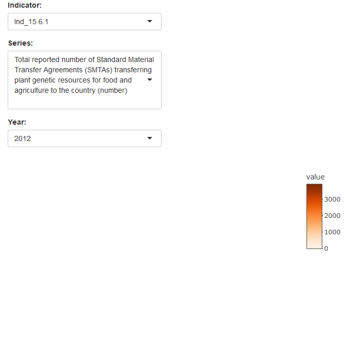

```

Matt

4 12 2020

Get the data