Using OpenAlex to get publication metadata

I have been playing around with the OpenAlexR package which interfaces with the OpenAlex API. This allows you to get bibliographic information about publications, authors, institutions, sources, funders, publishers, topics and concepts.

Here I first look at the proportion of open publications published by NINA over time.

First we need to look for the Institution ID.

library(openalexR, quietly = TRUE)
library(tidyverse, quietly = TRUE)

oa_fetch( entity = "inst", # same as "institutions" 
          display_name.search = "\"Norwegian Institute for Nature\"") |> 
  select(display_name, ror) |>  
  knitr::kable()

display_name	ror
Norwegian Institute for Nature Research	https://ror.org/04aha0598

Then we can get a dataframe of the publications.

All_NINA<- oa_fetch( entity = "works", institutions.ror = "04aha0598", type = "article", from_publication_date = "2000-01-01", is_paratext = "false" )

# Get the open records

open_access <- oa_fetch( entity = "works", institutions.ror = "04aha0598", type = "article", from_publication_date = "2000-01-01", is_paratext = "false", is_oa = "true", group_by = "publication_year" )

# Get the closed records
closed_access <- oa_fetch( entity = "works", institutions.ror = "04aha0598", type = "article", from_publication_date = "2000-01-01", is_paratext = "false", is_oa = "false", group_by = "publication_year" )

# Join the dataframes together
uf_df <- closed_access |>  
  select(- key_display_name) |>  
  full_join(open_access, by = "key", suffix = c("_ca", "_oa"))

Now we can plot the data.

uf_df  |>  filter(key <= 2024) |> # we do not yet have complete data for 2024
  pivot_longer(cols = starts_with("count"))  |> 
  mutate( year = as.integer(key), is_oa = recode( name, "count_ca" = "Closed Access", "count_oa" = "Open Access" ), label = if_else(key < 2024, NA_character_, is_oa) )  |> 
  select(year, value, is_oa, label)  |> 
  ggplot(aes(x = year, y = value, group = is_oa, color = is_oa)) + 
  geom_line(size = 1) + 
  labs( title = "NINA's progress towards Open Access", x = NULL, y = "Number of journal articles") +
  scale_color_brewer(palette = "Dark2", direction = -1) +
  scale_x_continuous(breaks = seq(2000, 2024, 2)) + 
  geom_text(aes(label = label), nudge_x = -5, hjust = 0) + 
  coord_cartesian(xlim = c(NA, 2024.5)) + 
  guides(color = "none")+ 
  ggthemes::theme_solarized()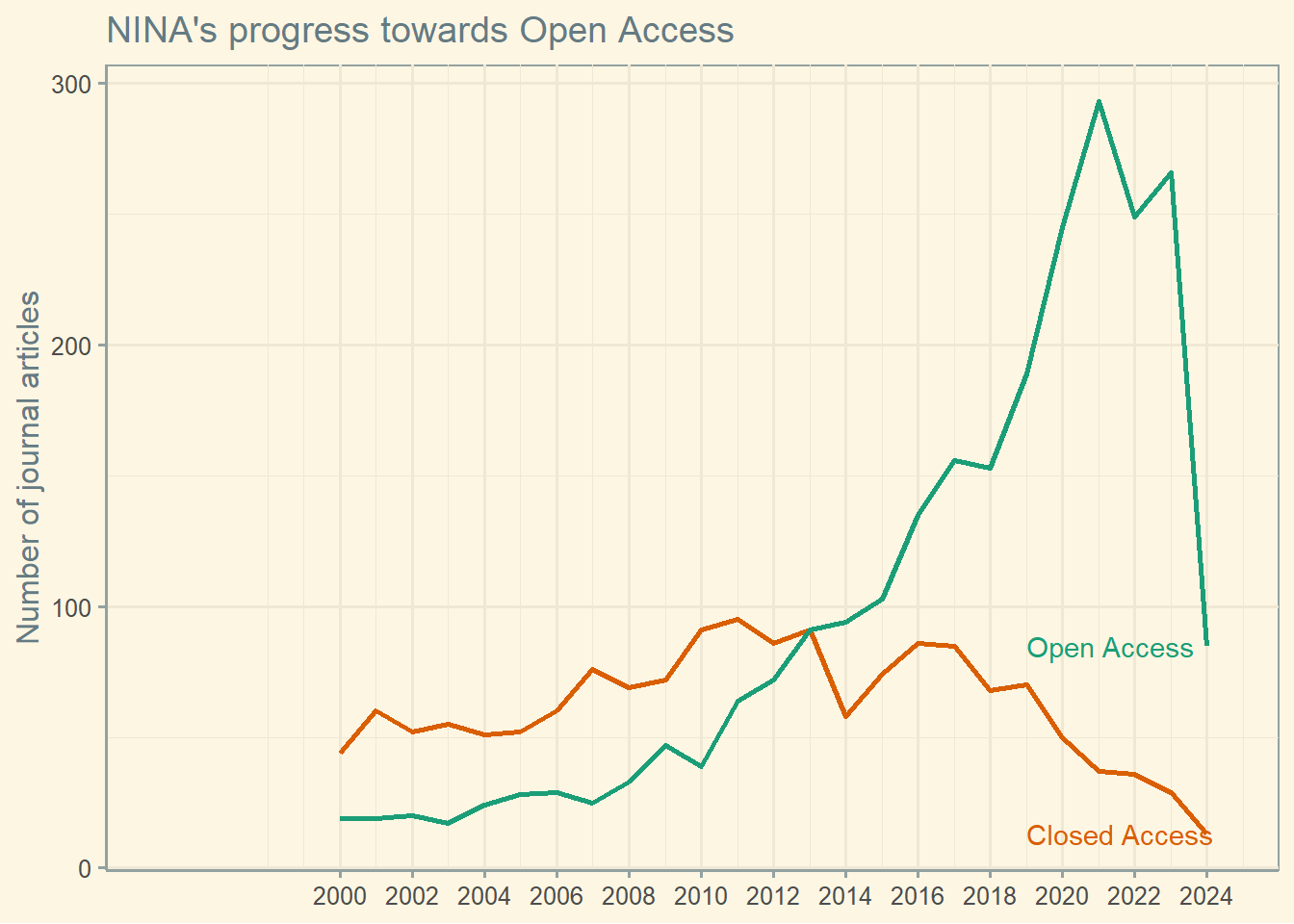

1 Extract the topics

The “topic” for each record is a description of the subject matter of the publication determined by using a large language model. The example from the OpenAlex topics page is:

Example Topic: “Artificial Intelligence in Medicine” Domain: “Health Sciences” Field: “Medicine” Subfield: “Health Informatics”

Each topic is made up of a subfield, a field and a domain. The model scores each documents topics, with the highest topic score being considered the “primary” topic.

1.1 All topics

expanded_tibble <- All_NINA |>  # Unnest the 'topics' to duplicate each row for each topic 
  unnest(topics, names_sep = "_")  |> 
  select(display_name, everything())

word_df<-expanded_tibble |> 
  group_by(topics_display_name) |> 
  tally()

wordcloud2::wordcloud2(word_df)

1.2 Primary topics

get_top_topic <- function(df) {
  if (nrow(df) == 0 || sum(df$name == "topic") == 0) {
    # If the dataframe is empty or contains no topics
    return(data.frame(display_name = NA, score = NA))
  } else {
    # Otherwise, proceed to get the top topic
    top_topic <- df  |> 
      filter(name == "topic")  |> 
      slice_max(order_by = score)  |> 
      slice_head(n = 1)  # Ensure only one result is returned
    return(top_topic)
  }
}

top_topics<-All_NINA  |> 
  mutate(
    top_topic_display_name = map_chr(topics, ~ {
      result <- get_top_topic(.x)
      if (nrow(result) > 0) result$display_name else NA
    }),
    top_topic_score = map_dbl(topics, ~ {
      result <- get_top_topic(.x)
      if (nrow(result) > 0) result$score else NA
    })
  )

topics_df<-top_topics |> 
  group_by(top_topic_display_name) |> 
  tally()

wordcloud2::wordcloud2(topics_df)