Code
library(tidyverse)
library(metafor)
library(patchwork)
set.seed(123)Funnel plots are one of the most widely used visual tools in meta-analysis. They are typically presented as a simple diagnostic for small-study effects or publication bias: if the plot is symmetric, things are fine; if it is asymmetric, something is wrong. This interpretation is already fragile (see this paper). In ecology, it is often incorrect.
Ecological meta-analyses rarely consist of independent, exchangeable study estimates. Instead, they are built from datasets with strong hierarchical structure: multiple effect sizes per study, shared controls, repeated measures, and outcomes that are intrinsically linked to study design and sample size.
When these data are plotted in a funnel plot, the resulting shape often reflects this structure rather than any underlying bias. In this post, I use simple simulations to show how funnel plot asymmetry can arise without any publication bias at all, and why visual interpretation is particularly misleading in ecological contexts.
library(tidyverse)
library(metafor)
library(patchwork)
set.seed(123)plot_funnel <- function(dat, title = "") {
# meta-analytic model
res <- rma(yi = yi, sei = sei, data = dat, method = "REML")
mu <- as.numeric(res$b)
sei_seq <- seq(min(dat$sei), max(dat$sei), length.out = 100)
funnel_df <- tibble(
sei = sei_seq,
left = mu - 1.96 * sei_seq,
right = mu + 1.96 * sei_seq
)
ggplot(dat, aes(x = yi, y = sei)) +
geom_point(alpha = 0.6) +
geom_line(data = funnel_df, aes(x = left, y = sei), linetype = "dashed") +
geom_line(data = funnel_df, aes(x = right, y = sei), linetype = "dashed") +
geom_vline(xintercept = mu) +
scale_y_reverse() +
labs(x = "Effect size", y = "Standard error", title = title) +
theme_minimal()
}We begin with the world that funnel plots assume: one independent effect size per study, with normally distributed sampling error.
n <- 40
theta <- rnorm(n, 0, 0.5)
sei <- runif(n, 0.1, 0.5)
yi <- rnorm(n, theta, sei)
dat1 <- tibble(yi, sei)
p1 <- plot_funnel(dat1, "1. Independent studies (no bias)")
p1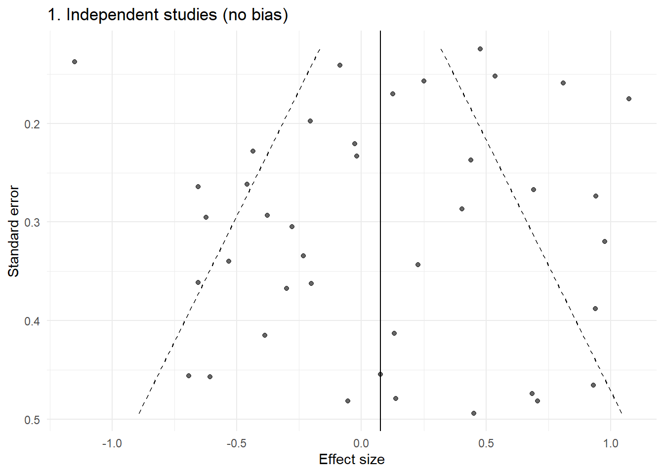
This is the idealised funnel: roughly symmetric, with increasing spread as precision decreases.
Now we introduce a simple selection mechanism: small, non-significant studies are less likely to be observed.
pvals <- 2 * pnorm(-abs(yi / sei))
keep <- !(sei > 0.3 & pvals > 0.05)
dat2 <- dat1[keep, ]
p2 <- plot_funnel(dat2, "2. Publication bias (textbook case)")
p2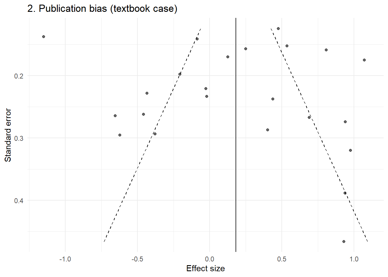
This produces the familiar asymmetric funnel that is typically interpreted as evidence of bias.
We now move into a more realistic ecological setting.
Each study contributes multiple effect sizes, sharing a common study-level effect.
n_study <- 40
effects_per_study <- sample(3:8, n_study, replace = TRUE)
dat3 <- map2_dfr(1:n_study, effects_per_study, function(j, k) {      u_j <- rnorm(1, 0, 0.5)
sei_j <- runif(1, 0.1, 0.4)
yi <- rnorm(k, u_j, sei_j)
tibble(     yi = yi,     sei = rep(sei_j, k),     study = j   ) })
p3 <- plot_funnel(dat3, "3. Hierarchical data (no bias)")
p3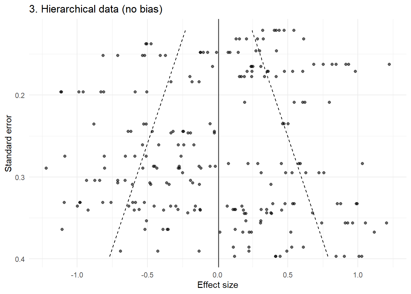
Even without any publication bias, the funnel now shows clear structure: clustering, banding, and apparent asymmetry.
This arises purely from non-independence.
Now we simulate multiple effect sizes derived from the same underlying sample (e.g. shared controls or repeated measures).
dat4 <- map2_dfr(1:n_study, effects_per_study, function(j, k) {      u_j <- rnorm(1, 0, 0.5)
base_se <- runif(1, 0.1, 0.3)
yi <- rnorm(k, u_j, base_se)
tibble(     yi = yi,     sei = rep(base_se, k),     study = j   ) })
p4 <- plot_funnel(dat4, "4. Shared controls / repeated measures")
p4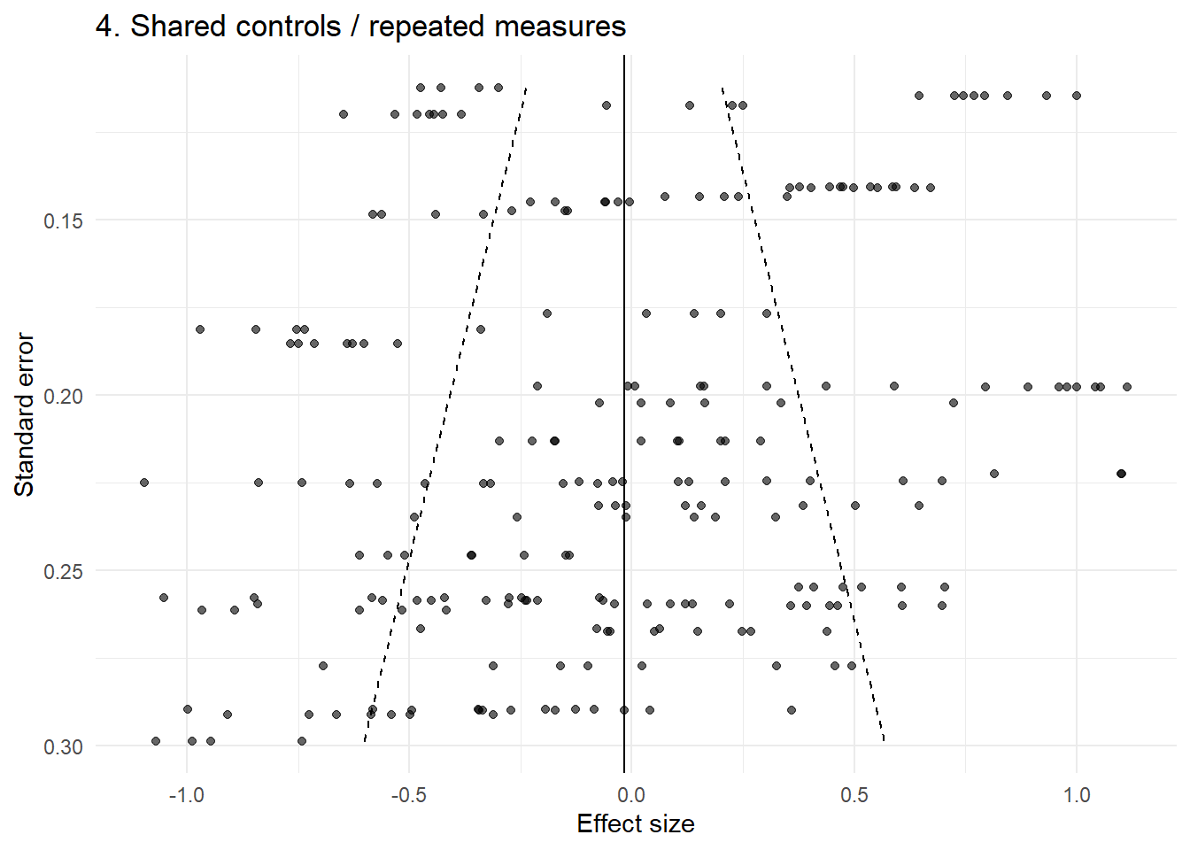
The funnel now develops bands and arcs, which are often misinterpreted as evidence of bias but are in fact artefacts of shared variance structure.
In many ecological datasets, study size is not random. Smaller studies may focus on particular systems, species, or experimental designs.
Here, we simulate a case where effect size is associated with study size.
n <- 80
sei <- runif(n, 0.1, 0.5)
theta <- 0.8 * (sei > 0.3) + rnorm(n, 0, 0.2)
yi <- rnorm(n, theta, sei)
dat5 <- tibble(yi, sei)
p5 <- plot_funnel(dat5, "5. Precision confounded with ecology")
p5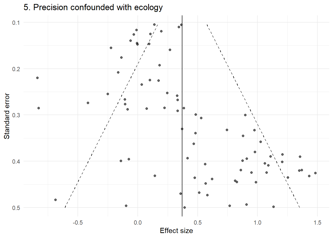
This produces clear asymmetry — but there is no publication bias. The pattern arises because small and large studies are studying different things.
Finally, we combine these features:
multiple effect sizes per study
shared precision within studies
strong heterogeneity
confounding between study size and effect
dat6 <- map2_dfr(1:n_study, effects_per_study, function(j, k) {      sei_j <- runif(1, 0.1, 0.4)
u_j <- rnorm(1, ifelse(sei_j > 0.25, 0.6, 0), 0.4)
yi <- rnorm(k, u_j, sei_j)
tibble(     yi = yi,     sei = rep(sei_j, k),     study = j   ) })
p6 <- plot_funnel(dat6, "6. Realistic ecological structure")
p6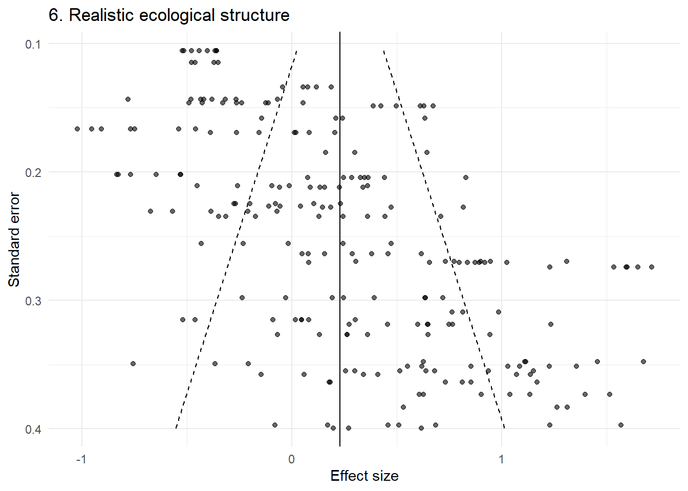
This looks highly structured and asymmetric — yet no publication bias has been introduced.
(p1 | p2) / (p3 | p4) / (p5 | p6)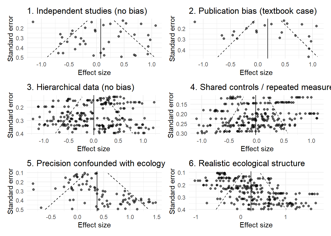
Across these examples, the key point is consistent:
The funnel plot is not simply reflecting missing studies. It is reflecting the structure of the data.
In ecological meta-analyses, that structure often includes:
multiple non-independent effect sizes per study
shared controls or repeated measures
study-level clustering
strong heterogeneity
relationships between study design and precision
Under these conditions, the assumptions underlying funnel plot interpretation are violated.
The usual advice is to “inspect the funnel plot for asymmetry.” However, this assumes that asymmetry primarily arises from small-study effects.
These simulations show that:
asymmetry can arise without any bias
structured patterns (bands, arcs, clusters) are common
visually striking funnels can be entirely artefactual
In this context, visual interpretation is not just subjective, it is often misleading.
Rather than relying on visual inspection of funnel plots, analyses should:
explicitly account for hierarchical structure
consider study-level aggregation as a sensitivity check
use multilevel meta-analytic models
explore moderators that may be confounded with precision
interpret any small-study effect diagnostics with extreme caution
Funnel plots were designed for a world of independent study estimates.
Ecological meta-analyses do not live in that world.
Before interpreting a funnel plot, we should first ask:
What structure do these points represent?
In many cases, the answer is not “a set of independent studies,” but a complex, hierarchical evidence base and the funnel plot is simply revealing that structure.
If ecologists want to explore whether effect sizes are associated with study precision, a more defensible approach is to use a multilevel meta-regression rather than relying on visual inspection of a raw funnel plot. This follows the general approach advocated by Nakagawa et al., who recommend modelling heterogeneity and non-independence directly, and then using residual funnel plots as a supplement rather than a primary diagnostic.
The idea is simple: if smaller or less precise studies tend to report systematically different effects, then effect size may be associated with sampling variance or standard error. In ecological meta-analysis, however, this association should be tested in a multilevel framework that reflects the dependency structure of the data.
library(dplyr)
library(purrr)
library(tibble)
library(metafor)
library(ggplot2)

set.seed(123)

# Assume your data look something like this:
# dat$yi        = effect size
# dat$vi        = sampling variance
# dat$study_id  = study identifier
# dat$obs_id    = effect-size identifier within study
# dat$year      = publication year (optional, for time-lag bias)

simulate_meta_ecology <- function(
  n_study = 40,
  min_es = 3,
  max_es = 8,
  tau = 0.5,              # between-study heterogeneity
  sigma_within = 0.2,     # within-study variation
  bias = FALSE,           # simulate publication bias
  confounding = FALSE,    # precision-effect confounding
  time_lag = FALSE        # time trend
) {

  # number of effect sizes per study
  n_es <- sample(min_es:max_es, n_study, replace = TRUE)

  dat <- map2_dfr(seq_len(n_study), n_es, function(j, k) {

    # study-level precision (shared within study)
    sei_j <- runif(1, 0.1, 0.5)
    vi_j  <- sei_j^2

    # study-level true effect
    if (confounding) {
      # less precise studies tend to have larger true effects
      mu_j <- rnorm(1, mean = ifelse(sei_j > 0.3, 0.6, 0), sd = tau)
    } else {
      mu_j <- rnorm(1, mean = 0, sd = tau)
    }

    # optional time trend
    year_j <- sample(1990:2020, 1)
    if (time_lag) {
      mu_j <- mu_j + 0.02 * (year_j - 2000)
    }

    # generate observed effect sizes
    yi <- rnorm(k, mean = mu_j, sd = sqrt(vi_j + sigma_within^2))

    tibble(
      yi = yi,
      vi = rep(vi_j, k),
      study_id = factor(j),
      obs_id = factor(paste0(j, "_", seq_len(k))),
      year = rep(year_j, k)
    )
  })

  # optional publication bias / small-study selection
  if (bias) {
    dat <- dat %>%
      mutate(
        sei = sqrt(vi),
        z = yi / sei,
        p = 2 * pnorm(-abs(z))
      ) %>%
      filter(!(sei > 0.3 & p > 0.05)) %>%
      select(-z, -p)
  }

  dat %>%
    mutate(sei = sqrt(vi))
}

# Simulate a dataset:
# - confounding = TRUE gives a precision-effect relationship without publication bias
# - time_lag = TRUE adds a publication year trend
dat <- simulate_meta_ecology(
  n_study = 40,
  min_es = 3,
  max_es = 8,
  tau = 0.5,
  sigma_within = 0.2,
  bias = FALSE,
  confounding = TRUE,
  time_lag = TRUE
)

# ---------------------------------------------------------
# Multilevel meta-analysis (baseline model)
# ---------------------------------------------------------

m0 <- rma.mv(
  yi = yi,
  V  = vi,
  random = ~ 1 | study_id/obs_id,
  data = dat,
  method = "REML"
)

summary(m0)
Multivariate Meta-Analysis Model (k = 209; method: REML)

   logLik   Deviance        AIC        BIC       AICc
-119.7124   239.4247   245.4247   255.4374   245.5424

Variance Components:

            estim    sqrt  nlvls  fixed           factor
sigma^2.1  0.3294  0.5740     40     no         study_id
sigma^2.2  0.0386  0.1963    209     no  study_id/obs_id

Test for Heterogeneity:
Q(df = 208) = 1758.9222, p-val < .0001

Model Results:

estimate      se    zval    pval   ci.lb   ci.ub
  0.4130  0.0947  4.3618  <.0001  0.2274  0.5986  ***

---
Signif. codes: 0 '***' 0.001 '**' 0.01 '*' 0.05 '.' 0.1 ' ' 1# ---------------------------------------------------------
# Multilevel small-study effect model
# (Egger-type meta-regression, but multilevel)
# ---------------------------------------------------------
m_pub <- rma.mv(
yi = yi,
V = vi,
mods = ~ sei,
random = ~ 1 | study_id/obs_id,
data = dat,
method = "REML"
)
summary(m_pub)
Multivariate Meta-Analysis Model (k = 209; method: REML)

   logLik   Deviance        AIC        BIC       AICc
-116.1614   232.3228   240.3228   253.6536   240.5208

Variance Components:

            estim    sqrt  nlvls  fixed           factor
sigma^2.1  0.2952  0.5433     40     no         study_id
sigma^2.2  0.0386  0.1964    209     no  study_id/obs_id

Test for Residual Heterogeneity:
QE(df = 207) = 1657.4039, p-val < .0001

Test of Moderators (coefficient 2):
QM(df = 1) = 4.9851, p-val = 0.0256

Model Results:

         estimate      se     zval    pval    ci.lb   ci.ub
intrcpt   -0.0773  0.2369  -0.3263  0.7442  -0.5416  0.3870
sei        1.7104  0.7660   2.2327  0.0256   0.2090  3.2118  *

---
Signif. codes: 0 '***' 0.001 '**' 0.01 '*' 0.05 '.' 0.1 ' ' 1# The coefficient for 'sei' is the key term:
# if it differs clearly from zero, effect size changes with precision,
# which is consistent with a small-study effect
# (but not necessarily publication bias)
# ---------------------------------------------------------
# Time-lag bias model
# ---------------------------------------------------------
m_time <- rma.mv(
yi = yi,
V = vi,
mods = ~ scale(year),
random = ~ 1 | study_id/obs_id,
data = dat,
method = "REML"
)
summary(m_time)
Multivariate Meta-Analysis Model (k = 209; method: REML)

   logLik   Deviance        AIC        BIC       AICc
-116.0127   232.0254   240.0254   253.3562   240.2234

Variance Components:

            estim    sqrt  nlvls  fixed           factor
sigma^2.1  0.2950  0.5431     40     no         study_id
sigma^2.2  0.0386  0.1964    209     no  study_id/obs_id

Test for Residual Heterogeneity:
QE(df = 207) = 1534.7321, p-val < .0001

Test of Moderators (coefficient 2):
QM(df = 1) = 5.2047, p-val = 0.0225

Model Results:

             estimate      se    zval    pval   ci.lb   ci.ub
intrcpt        0.4136  0.0900  4.5952  <.0001  0.2372  0.5901  ***
scale(year)    0.2098  0.0919  2.2814  0.0225  0.0296  0.3900    *

---
Signif. codes: 0 '***' 0.001 '**' 0.01 '*' 0.05 '.' 0.1 ' ' 1# ---------------------------------------------------------
# Residual funnel plot
# ---------------------------------------------------------
dat$resid_pub <- as.numeric(residuals(m_pub))
mu_resid <- 0
sei_seq <- seq(min(dat$sei), max(dat$sei), length.out = 200)
funnel_df <- tibble(
sei = sei_seq,
left = mu_resid - 1.96 * sei_seq,
right = mu_resid + 1.96 * sei_seq
)
ggplot(dat, aes(x = resid_pub, y = sei)) +
geom_point(alpha = 0.6) +
geom_line(data = funnel_df, aes(x = left, y = sei), linetype = "dashed") +
geom_line(data = funnel_df, aes(x = right, y = sei), linetype = "dashed") +
geom_vline(xintercept = 0) +
scale_y_reverse() +
labs(
x = "Residual effect size",
y = "Standard error",
title = "Residual funnel plot after multilevel meta-regression"
) +
theme_minimal()
This is not a magic solution. No publication-bias method is ideal in the kinds of hierarchical, heterogeneous datasets common in ecology, and Nakagawa et al. are very clear on that point. A multilevel meta-regression plus a residual funnel plot is much closer to the structure of ecological evidence than a visually interpreted raw funnel plot.