Flight summaries

Call in files from a nested folder and clean them

library(here)
#here::here()
path=paste0(here::here(),"/", "data/tables")
#list.files(path)
all_dfs=Kulan::get_tables(path, ".csv")
all_dfs=all_dfs %>% 
  janitor::clean_names() %>% 
  rename(., Flight = class)

#clean up the time format if needed (some issues with xls files)
# all_dfs <- all_dfs %>%
#             mutate(time = update(time,
#                        year = year(date),
#                        month = month(date),
#                        day = day(date)),
#             hms = hms::as_hms(time))

#Make sure values are recognized as numeric
all_dfs=all_dfs %>%
  mutate(banking_angle=as.numeric(banking_angle)) %>%
  mutate(tangage=as.numeric(tangage)) %>%
  mutate(azimuth=as.numeric(azimuth)) %>%
  mutate(gps_course=as.numeric(gps_course)) %>%
  mutate(speed=as.numeric(speed)) %>%
  mutate(gps_speed=as.numeric(gps_speed))

#shows if values are correctly defined
str(all_dfs)

## Classes 'data.table' and 'data.frame':   12670 obs. of  19 variables:
##  $ photo_no               : chr  "DSC06212.JPG" "DSC06213.JPG" "DSC06214.JPG" "DSC06215.JPG" ...
##  $ date                   : chr  "16.07.2020" "16.07.2020" "16.07.2020" "16.07.2020" ...
##  $ time                   : chr  "02:34:47" "02:34:50" "02:34:54" "02:37:42" ...
##  $ lat_dec                : num  45.8 45.8 45.8 45.8 45.8 ...
##  $ lon_dec                : num  61.2 61.2 61.2 61.2 61.2 ...
##  $ alt_above_the_sea_level: num  53.7 53.8 53.9 86.7 141.4 ...
##  $ alt_above_launch_point : num  0.4 0.5 0.2 37.9 91.5 ...
##  $ alt_above_ground       : num  0 0 0 33 87.7 ...
##  $ banking_angle          : num  -0.7 -1.6 0.1 -4.7 22.4 21.1 25.7 13.7 17.9 22.6 ...
##  $ tangage                : num  4 2.8 1.3 9.2 3.3 4 7 9.8 5.2 4.9 ...
##  $ azimuth                : num  75 75 76 74 85 162 227 297 10 88 ...
##  $ gps_course             : num  76.2 75.6 75.7 76.9 74.6 ...
##  $ speed                  : num  0 0 0 82.8 86 ...
##  $ gps_speed              : num  0 0 0 66.6 62.3 ...
##  $ camera_position        : chr  "right" "right" "right" "right" ...
##  $ species                : logi  NA NA NA NA NA NA ...
##  $ number                 : logi  NA NA NA NA NA NA ...
##  $ Flight                 : chr  "Flight1" "Flight1" "Flight1" "Flight1" ...
##  $ v18                    : logi  NA NA NA NA NA NA ...
##  - attr(*, ".internal.selfref")=<externalptr>

Extract raster values from a DEM for the altitude above ground calculations

At this point you could add the altitude from the DEM [see the “Getting raster values form a Digital Elevation Model” vignette]. Here, for this example, we will use the column called Altitude above the ground (because we can not include all the DEMs we would need inside the package).

Remove points where the drone is in take-off or landing

First plot the data

all_dfs %>% 
  mutate(time2=as.POSIXct(time,format="%H:%M:%S")) %>% 
  ggplot(aes(time2, alt_above_ground, colour=Flight))+ 
  geom_point()+
  labs(x="time",y= "Altitude above ground")+
  theme(legend.position = "None")+
  facet_wrap(~Flight)

## Warning: Removed 25 rows containing missing values (geom_point).

From the distribution of the altitudes we can see that anything below 200 m is probably take-off or landing phase.

all_dfs %>% 
  ggplot(aes(alt_above_ground))+
  geom_histogram(fill="Red")

## `stat_bin()` using `bins = 30`. Pick better value with `binwidth`.

## Warning: Removed 25 rows containing non-finite values (stat_bin).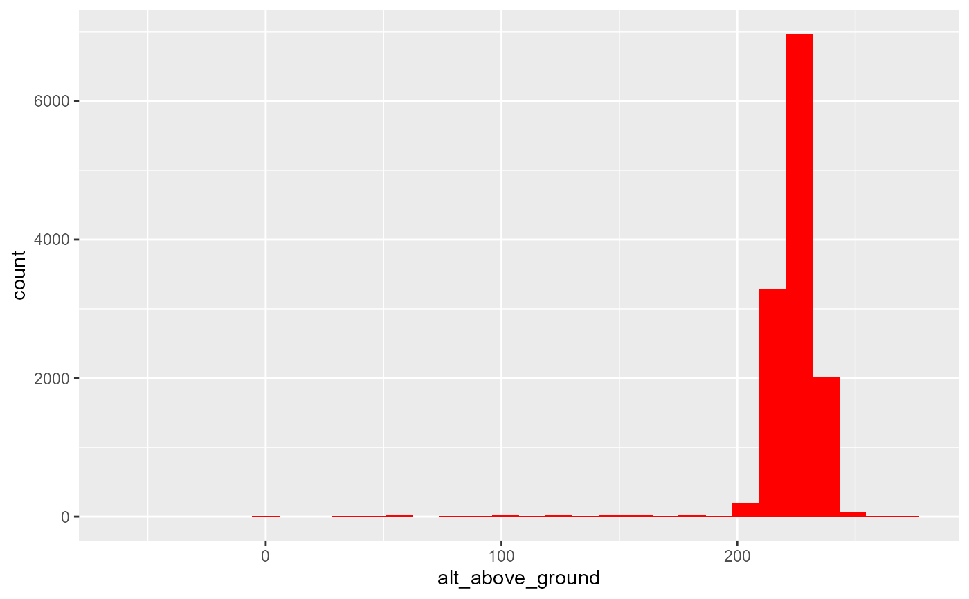

However, we might want to look more closely at Flight5 as it seems some of the points during the flight are below 200m.

all_dfs %>% 
  filter(Flight=="Flight5") %>% 
  ggplot(aes(time, alt_above_ground, colour=Flight)) +
  labs(y= "Altitude above sea level")+
  theme(axis.text.x = element_blank())+
  geom_point()+
  geom_hline(yintercept = 200, colour="Red", lty=2) +
  geom_hline(yintercept = 190, colour="Green", lty=2) +
  theme(legend.position = "None")

## Warning: Removed 4 rows containing missing values (geom_point).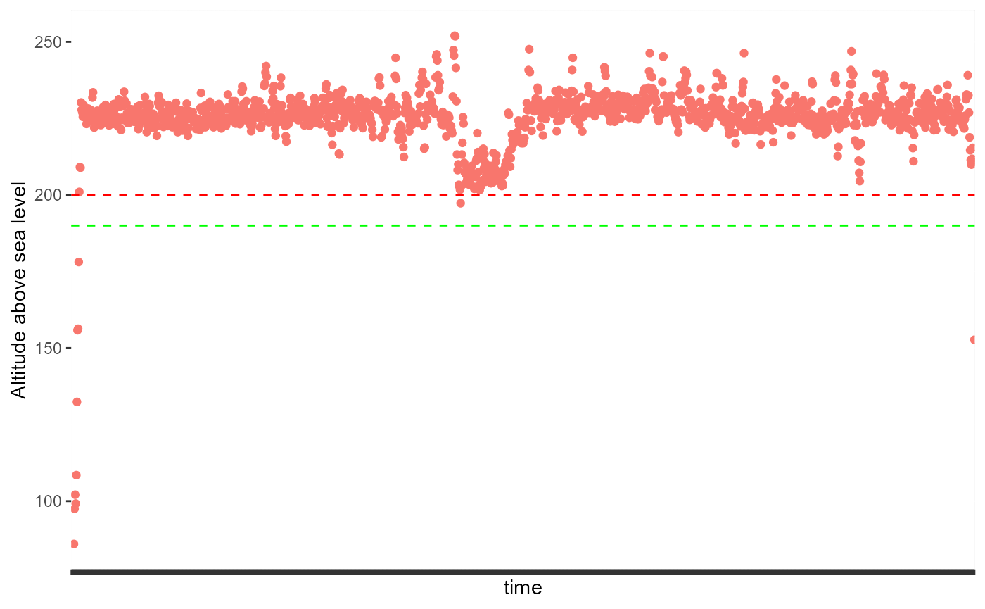

So a couple of points in Flight5 during the actual flight were below our threshold of 200m. So let’s be conservative and go for 190m instead. You can change this threshold by changing the value in the code below.

dfs_reduced=all_dfs %>% 
  filter(alt_above_ground>190)# The threshold is controlled here - change it by changing the number from 190

Now all the points in consideration are above 190m.

Drone flight descriptors

Altitude above ground summary

dfs_reduced %>% 
   mutate(time2=as.POSIXct(time,format="%H:%M:%S")) %>% 
  ggplot(aes(time2,alt_above_ground))+
  geom_point(colour="darkblue")+
  geom_line(colour="darkblue")+
  labs(x="time", y="Altitude above the ground")+
  facet_wrap(Flight~., scale="free")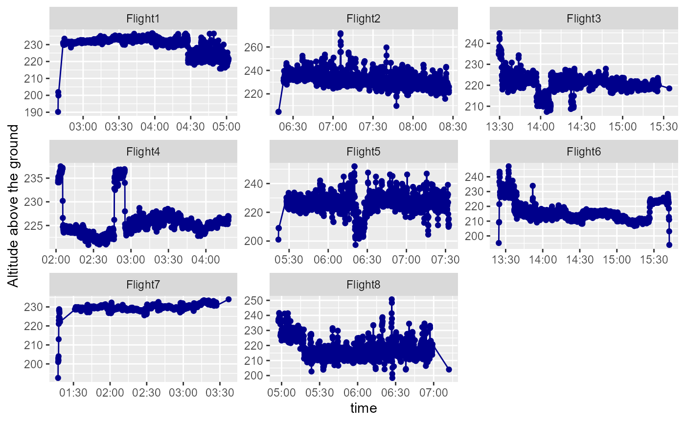

Trapeze - drone footprint for specific altitude example

#####################################################################################################################
# Drone & camera setup:
# Camera: SONY DCS-RX1RM2
# Sensor: 35.9 x 24.0 mm
# VIEWING ANGLE LENS (CORRESPONDING 35 MM FORMAT) 63 degrees (35mm))
# Image width in pixel: 7952
# Image height in pixel: 5304
# Camera angles 25.7 and 25.0 degrees
# distance between two lenses is 2,9-3,0 cm - this distance is in the forward direction 
# as both cameras are directly in the middle of the drone
#####################################################################################################################

library(patchwork)

## Warning: package 'patchwork' was built under R version 4.0.5

#short version of the below functions:
#Kulan::plot_trapezoid(altitude = 200, banking_angle = 0)

# calculat trapez based on drone specifications
# sensor and camera details
xsensor = 35.9   #sensor width
ysensor = 24     #sensor height
focallen    = 35     #focal length of lens
ygim        = 0      #roll
xgim1    = 25     #banking angle = camera angle 1
Xgim2   = 25.7   #banking angle = camera angle 2
alt         = 245    #fight height - change according to values seen under 4.3., I subsequently changed alt = alt, so it 
imW      = 7952   #sensor width
imH = 5304   #sensor length
#####################################################################################################################
#######################  5.2.1. trapeze side view
#####################################################################################################################
deg2rad<-function(d) {
  rad = d * pi / 180
  return(rad)
}

rad2deg<-function(rad) {
  deg=rad*180/pi
  return(deg)
}

FOV.wide<-rad2deg(2*atan(xsensor/(2*focallen)))
FOV.high<-rad2deg(2*atan(ysensor/(2*focallen)))

theta <- deg2rad(xgim1)
# horizontal field of view
phi <- deg2rad(FOV.wide)
# vertical field of view
omega <- deg2rad(FOV.high)

Dc = alt*tan(theta-phi/2)
Df = alt*tan(theta+phi/2)
Dm = alt*tan(theta+phi*0.5/2)

Rc = sqrt(alt^2+Dc^2)
Rm = sqrt(alt^2+Dm^2)
Rf = sqrt(alt^2+Df^2)

dt.triangle  <- data.table(group = c(1,1,1), polygon.x = c(0,Dc,0), polygon.y = c(alt,0,0))
dt.triangle2 <- data.table(group = c(1,1,1), polygon.x = c(0,Df,0), polygon.y = c(alt,0,0))

#plotting side view
p <- ggplot()
p <- p + geom_polygon(
  data = dt.triangle
  ,aes(
    x=polygon.x
    ,y=polygon.y
    ,group=group
  )
)
p+geom_polygon(
  data = dt.triangle2
  ,aes(
    x=polygon.x
    ,y=polygon.y
    ,group=group
    , alpha=0.2
  ))+
  labs(x="Horizontal distance", y="Vertical distance")+
  theme(legend.position = "None")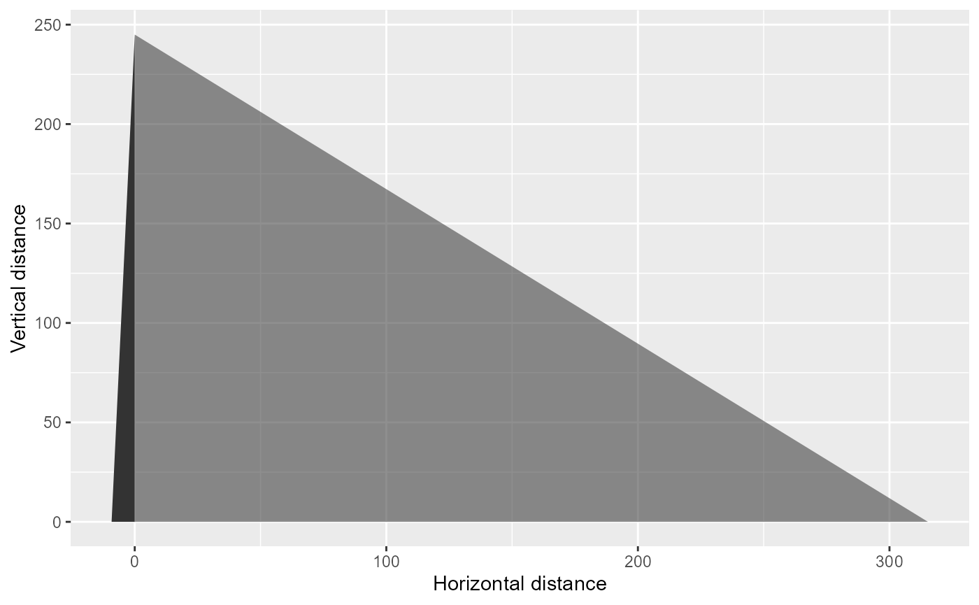

Adding the other camera

In our case we have two cameras with different angles and we can plot these to show the images horizontal footprints.

theta2 <- deg2rad(Xgim2)
Dc2 = alt*tan(theta2-phi/2)
Df2 = alt*tan(theta2+phi/2)
Dm2 = alt*tan(theta2+phi*0.5/2)

dt.triangle  <- data.table(group = c(1,1,1), polygon.x = c(0,Dc,0), polygon.y = c(alt,0,0))
dt.triangle2 <- data.table(group = c(1,1,1), polygon.x = c(0,Df,0), polygon.y = c(alt,0,0))

dt.triangle3 <- data.table(group = c(2,2,2), polygon.x3 = c(0,-Dc2,0), polygon.y3 = c(alt,0,0))
dt.triangle3 <- data.table(group = c(2,2,2), polygon.x3 = c(0,-Df2,0), polygon.y3 = c(alt,0,0))

p <- ggplot()
p <- p + geom_polygon(
  data = dt.triangle
  ,aes(
    x=polygon.x
    ,y=polygon.y
    ,group=group
  )
)
p<-p+geom_polygon(
  data = dt.triangle2
  ,aes(
    x=polygon.x
    ,y=polygon.y
    ,group=group
    , alpha=0.2
  ))
p+geom_polygon(
  data = dt.triangle3
  ,aes(
    x=polygon.x3
    ,y=polygon.y3
    ,group=group
    , alpha=0.2
  ))+
  labs(x="Horizontal distance", y="Vertical distance")+
  theme(legend.position = "None")

Trapeze top view

#Top view
Wc = 2*(Dc^2+alt^2)^0.5*tan(omega/2)
Wm = 2*((Dc+Df/2)^2+alt^2)^0.5*tan(omega/2)
Wf = 2*(Df^2+alt^2)^0.5*tan(omega/2)

positions <- data.frame(
  x = c(0, 0, Df-Dc, Df-Dc),
  y = c(-Wc/2, Wc/2, -Wf/2, Wf/2)
)
ggplot(positions[c(1,2,4,3),], aes(x = x, y = y)) +
  geom_polygon(aes(fill = "red"))+
  labs(x="", y="")+
  theme_classic()+
  theme(legend.position = "None")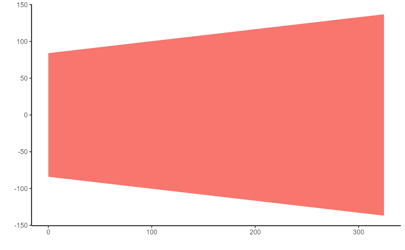

Strip-width summary

 dfs_reduced=dfs_reduced%>% 
    group_by(Flight) %>%
  filter(!str_detect(photo_no, "IMG")) %>% # remove empty photos
  rowwise() %>% 
  mutate("strip_width"=get_strip_width(alt=alt_above_ground,banking_angle = banking_angle)) %>% 
  drop_na(strip_width)
 our_summary1 <-
  list("strip width (m)" =
         list("min"       = ~ round(min(strip_width)),
              "max"       = ~ round(max(strip_width)),
              "mean (sd)" = ~qwraps2::mean_sd(strip_width)))


tab_1<-qwraps2::summary_table(dplyr::group_by(dfs_reduced, Flight),our_summary1)
tab_1

	Flight1 (N = 1665)	Flight2 (N = 1491)	Flight3 (N = 1407)	Flight4 (N = 1638)	Flight5 (N = 1498)	Flight6 (N = 1820)	Flight7 (N = 1443)	Flight8 (N = 1533)
strip width (m)
min	221	228	221	229	224	214	234	213
max	1069	1725	954	921	1205	965	1032	1194
mean (sd)	307.22 ± 41.72	316.14 ± 71.79	297.64 ± 49.41	300.94 ± 35.61	309.27 ± 63.06	290.50 ± 41.13	310.60 ± 55.21	296.27 ± 61.92

Speed summary

Using the gps_speed we can plot the speed of the drone during each flight.

dfs_reduced%>% 
  mutate(rowid=row_number()) %>% 
  mutate(time2=as.POSIXct(time,format="%H:%M:%S")) %>% 
  #ggplot(aes(time2,gps_speed))+# replace the next line with this to remove the alt_above_ground colour
  ggplot(aes(time2,gps_speed,colour=alt_above_ground))+
  geom_point()+
  geom_line()+
  labs(x="time", y="gps speed")+
  #geom_point(colour="darkblue")+# add these lines too and remove the two above
  #geom_line(colour="darkblue")+#
  facet_wrap(~Flight, scales="free")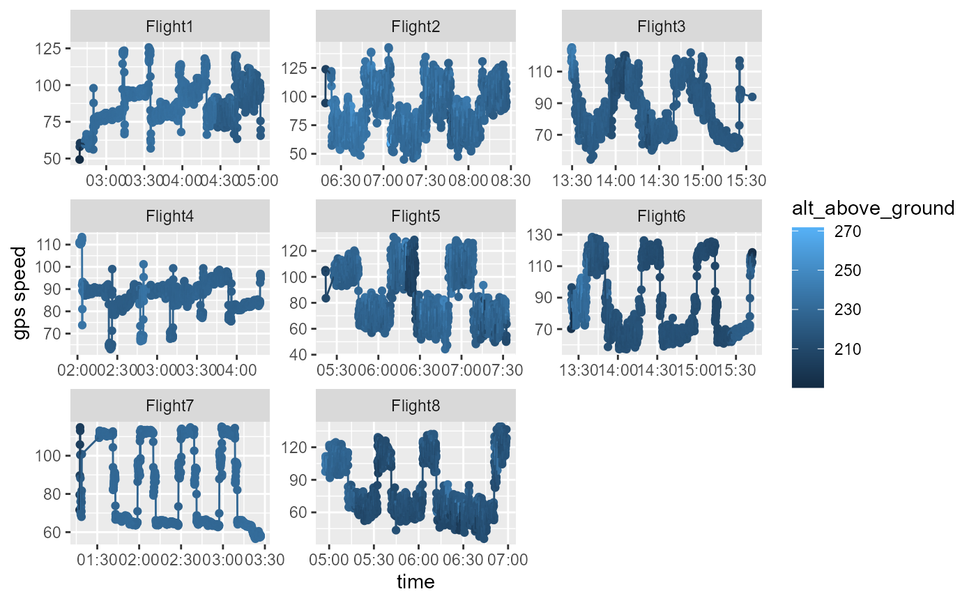

Distance between points summary

There are some very large distances moved at the start or the end of a Flight and these need to be filtered out to allow us to plot the distance more clearly. Anything above 250m is therefore removed in the plotting code below.The points are coloured by the gps_speed.

distance_df=dfs_reduced%>% 
  group_by(Flight) %>% 
  mutate(new_lat=lag(lat_dec)) %>%
  mutate(new_lon=lag(lon_dec)) %>%
  rowwise() %>%
  mutate(coord_dif=distm(c(lon_dec, lat_dec), c(new_lon, new_lat), fun = distHaversine))

distance_df %>% 
  group_by(Flight) %>% 
   mutate(time2=as.POSIXct(time,format="%H:%M:%S")) %>% 
  filter(coord_dif<250) %>% 
  ggplot(aes(time2,coord_dif,colour=coord_dif))+
  geom_point()+
  geom_line()+
  scale_colour_gradientn(colours = terrain.colors(10))+
  labs(x="time",y="distance (m) between points")+
  facet_wrap(~Flight, scales="free")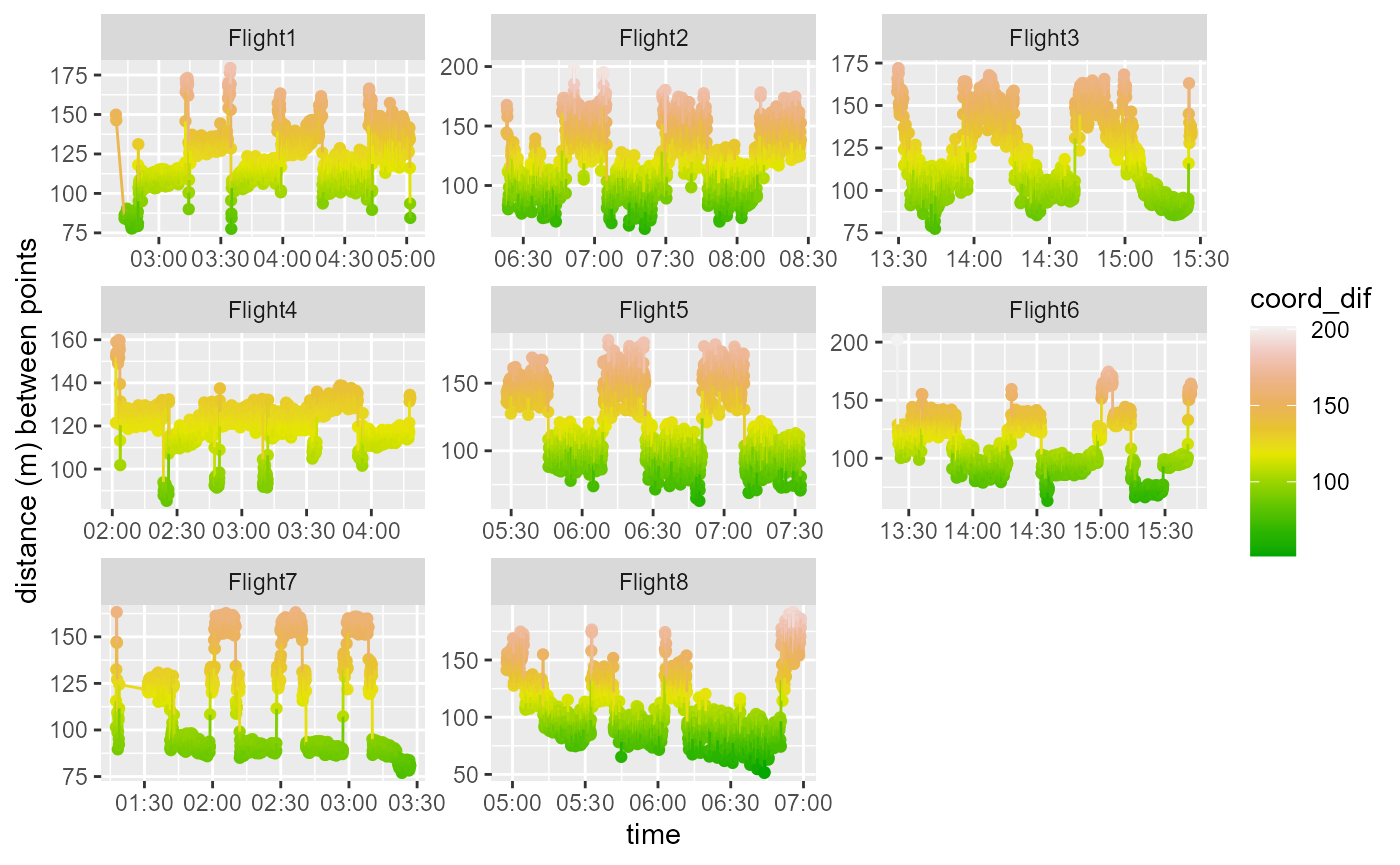

Banking Angle

dfs_reduced%>% 
  mutate(rowid=row_number()) %>% 
  mutate(time2=as.POSIXct(time,format="%H:%M:%S")) %>% 
  ggplot(aes(time2,banking_angle))+
  geom_point(colour="darkblue")+
  geom_line(colour="darkblue")+
  labs(x="time", y="Banking angle")+
  facet_wrap(~Flight, scales="free")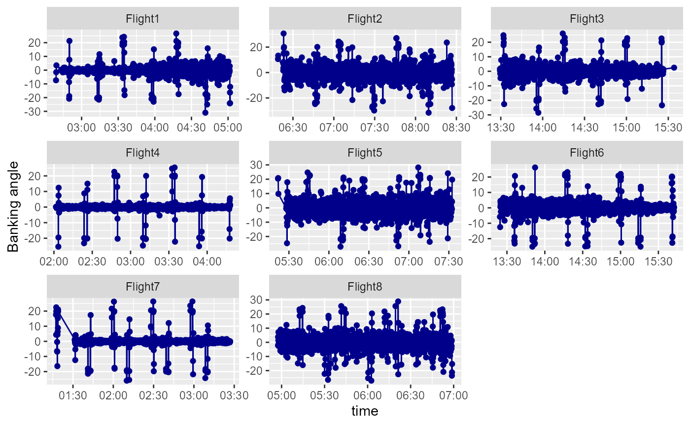

Photograph area on the right side

dfs_reduced=dfs_reduced %>% 
  rowwise() %>% 
  mutate("photo_area_R"=Kulan::get_photo_area(altitude = alt_above_ground,banking_angle = banking_angle))


dfs_reduced %>% 
  dplyr::select(photo_area_R) %>% 
  ggplot(aes(photo_area_R))+
  labs(x="photograph area m2")+
  geom_histogram(fill="red")+
  theme_classic()

## `stat_bin()` using `bins = 30`. Pick better value with `binwidth`.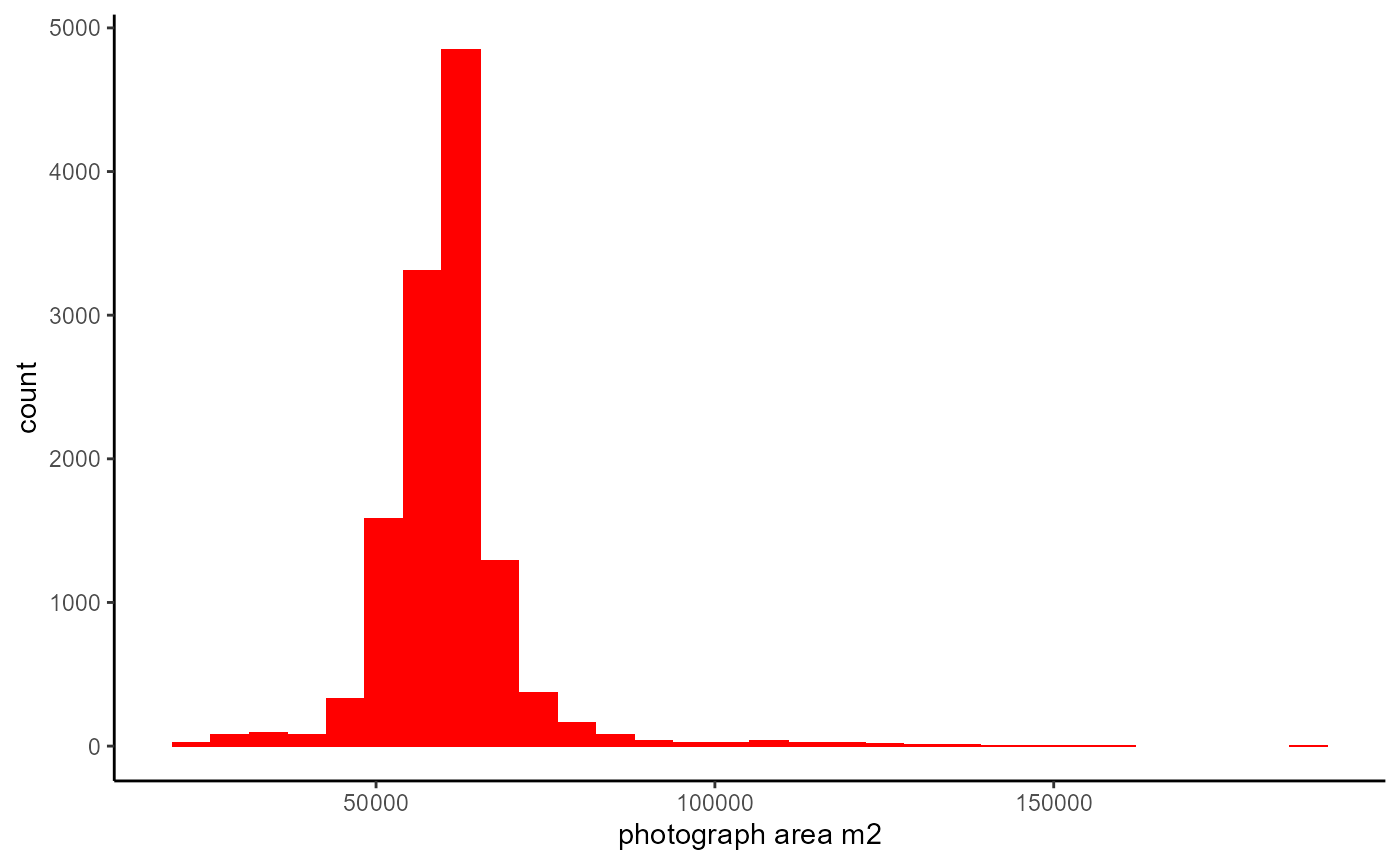

Photograph area on the left side

We need to change the camera angle from the default (which is set for the right side camera) in order to calculate the photo area on the left.

dfs_reduced=dfs_reduced %>% 
  rowwise() %>% 
  mutate("photo_area_L"=Kulan::get_photo_area(altitude = alt_above_ground, angle_of_camera = 25.7 ,banking_angle = banking_angle))


dfs_reduced %>% 
  dplyr::select(photo_area_L) %>% 
  ggplot(aes(photo_area_L))+
  labs(x="photograph area m2")+
  geom_histogram(fill="red")+
  theme_classic()

## `stat_bin()` using `bins = 30`. Pick better value with `binwidth`.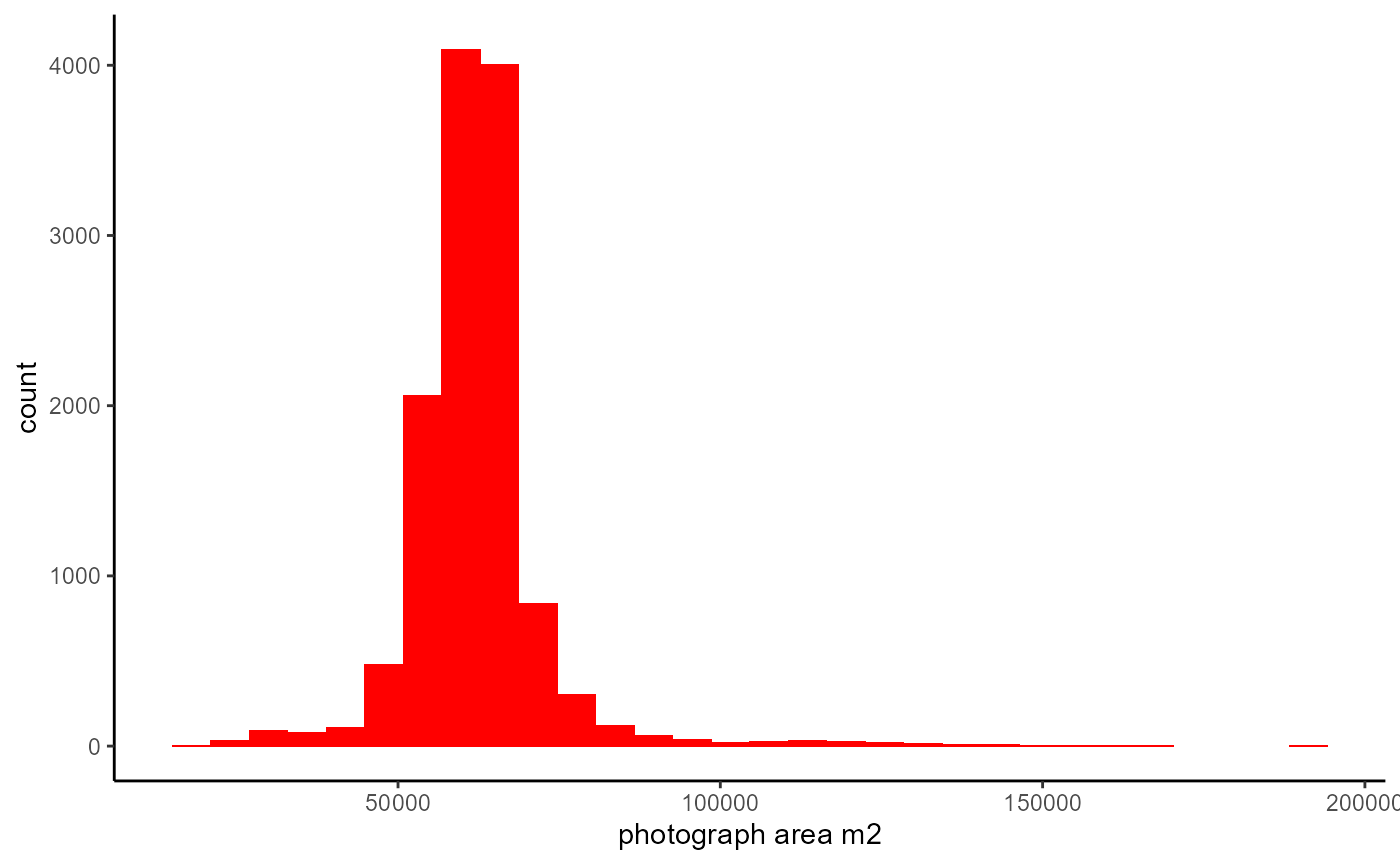

Overlap

The forward overlap is the percentage overlap that two consecutive images have. To calculate this value we could not use a single function so have developed a script to follow the process. This is hidden here in the rendered Markdown but contained in the script.

overlap_df=distance_df %>% 
  select(photo_no, alt_above_ground, coord_dif, banking_angle, Flight)

overlap_df$altitude1=overlap_df$alt_above_ground
overlap_df$altitude2=lead(overlap_df$altitude1)
overlap_df$distance=overlap_df$coord_dif
overlap_df$banking_angle1=overlap_df$banking_angle
overlap_df$banking_angle2=lead(overlap_df$banking_angle1)


overlap_df1=overlap_df %>%
  filter(Flight=="Flight1")

overlap_df1$forward_overlap=rep(NA,dim(overlap_df1)[1])


for (i in 2:dim(overlap_df1)[1]){

  altitude1=overlap_df1$altitude1[i]
  altitude2=overlap_df1$altitude2[i]
  forward_distance=overlap_df1$distance[i]
  angle_of_camera=25
  banking_angle1=overlap_df1$banking_angle1[i]
  banking_angle2=overlap_df1$banking_angle2[i]



  #Picture1
  h1=altitude1
  # angle of camera1
  theta1 <- Kulan::deg_to_rad(angle_of_camera)
  # horizontal field of view
  phi1 <- Kulan::deg_to_rad(Kulan::get_HFOV()+banking_angle1)
  # vertical field of view
  omega1 <- Kulan::deg_to_rad(Kulan::get_VFOV())
  Dc1= h1*tan(theta1-phi1/2)
  Df1= h1*tan(theta1+phi1/2)
  Dm1= h1*tan(theta1+phi1*0.5/2)
  Rc1=sqrt(h1^2+Dc1^2)
  Rm1=sqrt(h1^2+Dm1^2)
  Rf1=sqrt(h1^2+Df1^2)

  #Picture2
  h2=altitude2
  # angle of camera2
  theta2 <- Kulan::deg_to_rad(angle_of_camera)
  # horizontal field of view
  phi2 <- Kulan::deg_to_rad(Kulan::get_HFOV()+banking_angle2)
  # vertical field of view
  omega2 <- Kulan::deg_to_rad(Kulan::get_VFOV())
  Dc2= h2*tan(theta2-phi2/2)
  Df2= h2*tan(theta2+phi2/2)
  Dm2= h2*tan(theta2+phi2*0.5/2)
  Rc2=sqrt(h2^2+Dc2^2)
  Rm2=sqrt(h2^2+Dm2^2)
  Rf2=sqrt(h2^2+Df2^2)

  #Work out overlap between trapezoids
  Wc1=2*(Dc1^2+h1^2)^0.5*tan(omega1/2)
  Wm1=2*((Dc1+Df1/2)^2+h1^2)^0.5*tan(omega1/2)
  Wf1=2*(Df1^2+h1^2)^0.5*tan(omega1/2)
  positions1 <- data.frame(
    x = c(0, 0, Df1-Dc1, Df1-Dc1),
    y = c(-Wc1/2, Wc1/2, -Wf1/2, Wf1/2)
  )

  Wc2=2*(Dc2^2+h2^2)^0.5*tan(omega2/2)
  Wm2=2*((Dc2+Df2/2)^2+h2^2)^0.5*tan(omega2/2)
  Wf2=2*(Df2^2+h2^2)^0.5*tan(omega2/2)
  positions2 <- data.frame(
    x = c(0, 0, Df2-Dc2, Df2-Dc2),
    y = c(-Wc2/2+forward_distance, Wc2/2+forward_distance,
          -Wf2/2+forward_distance, Wf2/2+forward_distance)
  )

  library(sp)
  p = Polygon(positions1[c(1,2,4,3),] )
  ps = Polygons(list(p),1)
  sps = SpatialPolygons(list(ps))
  p2 = Polygon(positions2[c(1,2,4,3),] )
  ps2 = Polygons(list(p2),1)
  sps2 = SpatialPolygons(list(ps2))
  #plot(rgeos::gIntersection(sps,sps2), add=TRUE)
  area=rgeos::gIntersection(sps,sps2)
  if(is.null(area)){
    overlap_df1$forward_overlap[i]=0
  }else{
  overlap_df1$forward_overlap[i]=area@polygons[[1]]@area
  }
}

## Warning: package 'sp' was built under R version 4.0.5

overlap_df1$forward_overlap

###############################################################

overlap_df2=overlap_df %>%
  filter(Flight=="Flight2")

overlap_df2$forward_overlap=rep(NA,dim(overlap_df2)[1])


for (i in 2:dim(overlap_df2)[1]){

  altitude1=overlap_df2$altitude1[i]
  altitude2=overlap_df2$altitude2[i]
  forward_distance=overlap_df2$distance[i]
  angle_of_camera=25
  banking_angle1=overlap_df2$banking_angle1[i]
  banking_angle2=overlap_df2$banking_angle2[i]



  #Picture1
  h1=altitude1
  # angle of camera1
  theta1 <- Kulan::deg_to_rad(angle_of_camera)
  # horizontal field of view
  phi1 <- Kulan::deg_to_rad(Kulan::get_HFOV()+banking_angle1)
  # vertical field of view
  omega1 <- Kulan::deg_to_rad(Kulan::get_VFOV())
  Dc1= h1*tan(theta1-phi1/2)
  Df1= h1*tan(theta1+phi1/2)
  Dm1= h1*tan(theta1+phi1*0.5/2)
  Rc1=sqrt(h1^2+Dc1^2)
  Rm1=sqrt(h1^2+Dm1^2)
  Rf1=sqrt(h1^2+Df1^2)

  #Picture2
  h2=altitude2
  # angle of camera2
  theta2 <- Kulan::deg_to_rad(angle_of_camera)
  # horizontal field of view
  phi2 <- Kulan::deg_to_rad(Kulan::get_HFOV()+banking_angle2)
  # vertical field of view
  omega2 <- Kulan::deg_to_rad(Kulan::get_VFOV())
  Dc2= h2*tan(theta2-phi2/2)
  Df2= h2*tan(theta2+phi2/2)
  Dm2= h2*tan(theta2+phi2*0.5/2)
  Rc2=sqrt(h2^2+Dc2^2)
  Rm2=sqrt(h2^2+Dm2^2)
  Rf2=sqrt(h2^2+Df2^2)

  #Work out overlap between trapezoids
  Wc1=2*(Dc1^2+h1^2)^0.5*tan(omega1/2)
  Wm1=2*((Dc1+Df1/2)^2+h1^2)^0.5*tan(omega1/2)
  Wf1=2*(Df1^2+h1^2)^0.5*tan(omega1/2)
  positions1 <- data.frame(
    x = c(0, 0, Df1-Dc1, Df1-Dc1),
    y = c(-Wc1/2, Wc1/2, -Wf1/2, Wf1/2)
  )

  Wc2=2*(Dc2^2+h2^2)^0.5*tan(omega2/2)
  Wm2=2*((Dc2+Df2/2)^2+h2^2)^0.5*tan(omega2/2)
  Wf2=2*(Df2^2+h2^2)^0.5*tan(omega2/2)
  positions2 <- data.frame(
    x = c(0, 0, Df2-Dc2, Df2-Dc2),
    y = c(-Wc2/2+forward_distance, Wc2/2+forward_distance,
          -Wf2/2+forward_distance, Wf2/2+forward_distance)
  )

  library(sp)
  p = Polygon(positions1[c(1,2,4,3),] )
  ps = Polygons(list(p),1)
  sps = SpatialPolygons(list(ps))
  p2 = Polygon(positions2[c(1,2,4,3),] )
  ps2 = Polygons(list(p2),1)
  sps2 = SpatialPolygons(list(ps2))
  #plot(rgeos::gIntersection(sps,sps2), add=TRUE)
  area=rgeos::gIntersection(sps,sps2)
  if(is.null(area)){
    overlap_df2$forward_overlap[i]=0
  }else{
    overlap_df2$forward_overlap[i]=area@polygons[[1]]@area
  }
}
overlap_df2$forward_overlap

########################################################
overlap_df3=overlap_df %>%
  filter(Flight=="Flight3")

overlap_df3$forward_overlap=rep(NA,dim(overlap_df3)[1])


for (i in 2:dim(overlap_df3)[1]){

  altitude1=overlap_df3$altitude1[i]
  altitude2=overlap_df3$altitude2[i]
  forward_distance=overlap_df3$distance[i]
  angle_of_camera=25
  banking_angle1=overlap_df3$banking_angle1[i]
  banking_angle2=overlap_df3$banking_angle2[i]



  #Picture1
  h1=altitude1
  # angle of camera1
  theta1 <- Kulan::deg_to_rad(angle_of_camera)
  # horizontal field of view
  phi1 <- Kulan::deg_to_rad(Kulan::get_HFOV()+banking_angle1)
  # vertical field of view
  omega1 <- Kulan::deg_to_rad(Kulan::get_VFOV())
  Dc1= h1*tan(theta1-phi1/2)
  Df1= h1*tan(theta1+phi1/2)
  Dm1= h1*tan(theta1+phi1*0.5/2)
  Rc1=sqrt(h1^2+Dc1^2)
  Rm1=sqrt(h1^2+Dm1^2)
  Rf1=sqrt(h1^2+Df1^2)

  #Picture2
  h2=altitude2
  # angle of camera2
  theta2 <- Kulan::deg_to_rad(angle_of_camera)
  # horizontal field of view
  phi2 <- Kulan::deg_to_rad(Kulan::get_HFOV()+banking_angle2)
  # vertical field of view
  omega2 <- Kulan::deg_to_rad(Kulan::get_VFOV())
  Dc2= h2*tan(theta2-phi2/2)
  Df2= h2*tan(theta2+phi2/2)
  Dm2= h2*tan(theta2+phi2*0.5/2)
  Rc2=sqrt(h2^2+Dc2^2)
  Rm2=sqrt(h2^2+Dm2^2)
  Rf2=sqrt(h2^2+Df2^2)

  #Work out overlap between trapezoids
  Wc1=2*(Dc1^2+h1^2)^0.5*tan(omega1/2)
  Wm1=2*((Dc1+Df1/2)^2+h1^2)^0.5*tan(omega1/2)
  Wf1=2*(Df1^2+h1^2)^0.5*tan(omega1/2)
  positions1 <- data.frame(
    x = c(0, 0, Df1-Dc1, Df1-Dc1),
    y = c(-Wc1/2, Wc1/2, -Wf1/2, Wf1/2)
  )

  Wc2=2*(Dc2^2+h2^2)^0.5*tan(omega2/2)
  Wm2=2*((Dc2+Df2/2)^2+h2^2)^0.5*tan(omega2/2)
  Wf2=2*(Df2^2+h2^2)^0.5*tan(omega2/2)
  positions2 <- data.frame(
    x = c(0, 0, Df2-Dc2, Df2-Dc2),
    y = c(-Wc2/2+forward_distance, Wc2/2+forward_distance,
          -Wf2/2+forward_distance, Wf2/2+forward_distance)
  )

  library(sp)
  p = Polygon(positions1[c(1,2,4,3),] )
  ps = Polygons(list(p),1)
  sps = SpatialPolygons(list(ps))
  p2 = Polygon(positions2[c(1,2,4,3),] )
  ps2 = Polygons(list(p2),1)
  sps2 = SpatialPolygons(list(ps2))
  #plot(rgeos::gIntersection(sps,sps2), add=TRUE)
  area=rgeos::gIntersection(sps,sps2)
  if(is.null(area)){
    overlap_df3$forward_overlap[i]=0
  }else{
    overlap_df3$forward_overlap[i]=area@polygons[[1]]@area
  }
}
overlap_df3$forward_overlap

###########################################################

overlap_df4=overlap_df %>%
  filter(Flight=="Flight4")

overlap_df4$forward_overlap=rep(NA,dim(overlap_df4)[1])

for (i in 2:dim(overlap_df4)[1]){

  altitude1=overlap_df4$altitude1[i]
  altitude2=overlap_df4$altitude2[i]
  forward_distance=overlap_df4$distance[i]
  angle_of_camera=25
  banking_angle1=overlap_df4$banking_angle1[i]
  banking_angle2=overlap_df4$banking_angle2[i]



  #Picture1
  h1=altitude1
  # angle of camera1
  theta1 <- Kulan::deg_to_rad(angle_of_camera)
  # horizontal field of view
  phi1 <- Kulan::deg_to_rad(Kulan::get_HFOV()+banking_angle1)
  # vertical field of view
  omega1 <- Kulan::deg_to_rad(Kulan::get_VFOV())
  Dc1= h1*tan(theta1-phi1/2)
  Df1= h1*tan(theta1+phi1/2)
  Dm1= h1*tan(theta1+phi1*0.5/2)
  Rc1=sqrt(h1^2+Dc1^2)
  Rm1=sqrt(h1^2+Dm1^2)
  Rf1=sqrt(h1^2+Df1^2)

  #Picture2
  h2=altitude2
  # angle of camera2
  theta2 <- Kulan::deg_to_rad(angle_of_camera)
  # horizontal field of view
  phi2 <- Kulan::deg_to_rad(Kulan::get_HFOV()+banking_angle2)
  # vertical field of view
  omega2 <- Kulan::deg_to_rad(Kulan::get_VFOV())
  Dc2= h2*tan(theta2-phi2/2)
  Df2= h2*tan(theta2+phi2/2)
  Dm2= h2*tan(theta2+phi2*0.5/2)
  Rc2=sqrt(h2^2+Dc2^2)
  Rm2=sqrt(h2^2+Dm2^2)
  Rf2=sqrt(h2^2+Df2^2)

  #Work out overlap between trapezoids
  Wc1=2*(Dc1^2+h1^2)^0.5*tan(omega1/2)
  Wm1=2*((Dc1+Df1/2)^2+h1^2)^0.5*tan(omega1/2)
  Wf1=2*(Df1^2+h1^2)^0.5*tan(omega1/2)
  positions1 <- data.frame(
    x = c(0, 0, Df1-Dc1, Df1-Dc1),
    y = c(-Wc1/2, Wc1/2, -Wf1/2, Wf1/2)
  )

  Wc2=2*(Dc2^2+h2^2)^0.5*tan(omega2/2)
  Wm2=2*((Dc2+Df2/2)^2+h2^2)^0.5*tan(omega2/2)
  Wf2=2*(Df2^2+h2^2)^0.5*tan(omega2/2)
  positions2 <- data.frame(
    x = c(0, 0, Df2-Dc2, Df2-Dc2),
    y = c(-Wc2/2+forward_distance, Wc2/2+forward_distance,
          -Wf2/2+forward_distance, Wf2/2+forward_distance)
  )

  library(sp)
  p = Polygon(positions1[c(1,2,4,3),] )
  ps = Polygons(list(p),1)
  sps = SpatialPolygons(list(ps))
  p2 = Polygon(positions2[c(1,2,4,3),] )
  ps2 = Polygons(list(p2),1)
  sps2 = SpatialPolygons(list(ps2))
  #plot(rgeos::gIntersection(sps,sps2), add=TRUE)
  area=rgeos::gIntersection(sps,sps2)
  if(is.null(area)){
    overlap_df4$forward_overlap[i]=0
  }else{
    overlap_df4$forward_overlap[i]=area@polygons[[1]]@area
  }
}
overlap_df4$forward_overlap

###############################################################
overlap_df5=overlap_df %>%
  filter(Flight=="Flight5")

overlap_df5$forward_overlap=rep(NA,dim(overlap_df5)[1])


for (i in 2:dim(overlap_df5)[1]){

  altitude1=overlap_df5$altitude1[i]
  altitude2=overlap_df5$altitude2[i]
  forward_distance=overlap_df5$distance[i]
  angle_of_camera=25
  banking_angle1=overlap_df5$banking_angle1[i]
  banking_angle2=overlap_df5$banking_angle2[i]



  #Picture1
  h1=altitude1
  # angle of camera1
  theta1 <- Kulan::deg_to_rad(angle_of_camera)
  # horizontal field of view
  phi1 <- Kulan::deg_to_rad(Kulan::get_HFOV()+banking_angle1)
  # vertical field of view
  omega1 <- Kulan::deg_to_rad(Kulan::get_VFOV())
  Dc1= h1*tan(theta1-phi1/2)
  Df1= h1*tan(theta1+phi1/2)
  Dm1= h1*tan(theta1+phi1*0.5/2)
  Rc1=sqrt(h1^2+Dc1^2)
  Rm1=sqrt(h1^2+Dm1^2)
  Rf1=sqrt(h1^2+Df1^2)

  #Picture2
  h2=altitude2
  # angle of camera2
  theta2 <- Kulan::deg_to_rad(angle_of_camera)
  # horizontal field of view
  phi2 <- Kulan::deg_to_rad(Kulan::get_HFOV()+banking_angle2)
  # vertical field of view
  omega2 <- Kulan::deg_to_rad(Kulan::get_VFOV())
  Dc2= h2*tan(theta2-phi2/2)
  Df2= h2*tan(theta2+phi2/2)
  Dm2= h2*tan(theta2+phi2*0.5/2)
  Rc2=sqrt(h2^2+Dc2^2)
  Rm2=sqrt(h2^2+Dm2^2)
  Rf2=sqrt(h2^2+Df2^2)

  #Work out overlap between trapezoids
  Wc1=2*(Dc1^2+h1^2)^0.5*tan(omega1/2)
  Wm1=2*((Dc1+Df1/2)^2+h1^2)^0.5*tan(omega1/2)
  Wf1=2*(Df1^2+h1^2)^0.5*tan(omega1/2)
  positions1 <- data.frame(
    x = c(0, 0, Df1-Dc1, Df1-Dc1),
    y = c(-Wc1/2, Wc1/2, -Wf1/2, Wf1/2)
  )

  Wc2=2*(Dc2^2+h2^2)^0.5*tan(omega2/2)
  Wm2=2*((Dc2+Df2/2)^2+h2^2)^0.5*tan(omega2/2)
  Wf2=2*(Df2^2+h2^2)^0.5*tan(omega2/2)
  positions2 <- data.frame(
    x = c(0, 0, Df2-Dc2, Df2-Dc2),
    y = c(-Wc2/2+forward_distance, Wc2/2+forward_distance,
          -Wf2/2+forward_distance, Wf2/2+forward_distance)
  )

  library(sp)
  p = Polygon(positions1[c(1,2,4,3),] )
  ps = Polygons(list(p),1)
  sps = SpatialPolygons(list(ps))
  p2 = Polygon(positions2[c(1,2,4,3),] )
  ps2 = Polygons(list(p2),1)
  sps2 = SpatialPolygons(list(ps2))
  #plot(rgeos::gIntersection(sps,sps2), add=TRUE)
  area=rgeos::gIntersection(sps,sps2)
  if(is.null(area)){
    overlap_df5$forward_overlap[i]=0
  }else{
    overlap_df5$forward_overlap[i]=area@polygons[[1]]@area
  }
}
overlap_df5$forward_overlap

################################################################
overlap_df6=overlap_df %>%
  filter(Flight=="Flight6")

overlap_df6$forward_overlap=rep(NA,dim(overlap_df6)[1])


for (i in 2:dim(overlap_df6)[1]){

  altitude1=overlap_df6$altitude1[i]
  altitude2=overlap_df6$altitude2[i]
  forward_distance=overlap_df6$distance[i]
  angle_of_camera=25
  banking_angle1=overlap_df6$banking_angle1[i]
  banking_angle2=overlap_df6$banking_angle2[i]



  #Picture1
  h1=altitude1
  # angle of camera1
  theta1 <- Kulan::deg_to_rad(angle_of_camera)
  # horizontal field of view
  phi1 <- Kulan::deg_to_rad(Kulan::get_HFOV()+banking_angle1)
  # vertical field of view
  omega1 <- Kulan::deg_to_rad(Kulan::get_VFOV())
  Dc1= h1*tan(theta1-phi1/2)
  Df1= h1*tan(theta1+phi1/2)
  Dm1= h1*tan(theta1+phi1*0.5/2)
  Rc1=sqrt(h1^2+Dc1^2)
  Rm1=sqrt(h1^2+Dm1^2)
  Rf1=sqrt(h1^2+Df1^2)

  #Picture2
  h2=altitude2
  # angle of camera2
  theta2 <- Kulan::deg_to_rad(angle_of_camera)
  # horizontal field of view
  phi2 <- Kulan::deg_to_rad(Kulan::get_HFOV()+banking_angle2)
  # vertical field of view
  omega2 <- Kulan::deg_to_rad(Kulan::get_VFOV())
  Dc2= h2*tan(theta2-phi2/2)
  Df2= h2*tan(theta2+phi2/2)
  Dm2= h2*tan(theta2+phi2*0.5/2)
  Rc2=sqrt(h2^2+Dc2^2)
  Rm2=sqrt(h2^2+Dm2^2)
  Rf2=sqrt(h2^2+Df2^2)

  #Work out overlap between trapezoids
  Wc1=2*(Dc1^2+h1^2)^0.5*tan(omega1/2)
  Wm1=2*((Dc1+Df1/2)^2+h1^2)^0.5*tan(omega1/2)
  Wf1=2*(Df1^2+h1^2)^0.5*tan(omega1/2)
  positions1 <- data.frame(
    x = c(0, 0, Df1-Dc1, Df1-Dc1),
    y = c(-Wc1/2, Wc1/2, -Wf1/2, Wf1/2)
  )

  Wc2=2*(Dc2^2+h2^2)^0.5*tan(omega2/2)
  Wm2=2*((Dc2+Df2/2)^2+h2^2)^0.5*tan(omega2/2)
  Wf2=2*(Df2^2+h2^2)^0.5*tan(omega2/2)
  positions2 <- data.frame(
    x = c(0, 0, Df2-Dc2, Df2-Dc2),
    y = c(-Wc2/2+forward_distance, Wc2/2+forward_distance,
          -Wf2/2+forward_distance, Wf2/2+forward_distance)
  )

  library(sp)
  p = Polygon(positions1[c(1,2,4,3),] )
  ps = Polygons(list(p),1)
  sps = SpatialPolygons(list(ps))
  p2 = Polygon(positions2[c(1,2,4,3),] )
  ps2 = Polygons(list(p2),1)
  sps2 = SpatialPolygons(list(ps2))
  #plot(rgeos::gIntersection(sps,sps2), add=TRUE)
  area=rgeos::gIntersection(sps,sps2)
  if(is.null(area)){
    overlap_df6$forward_overlap[i]=0
  }else{
    overlap_df6$forward_overlap[i]=area@polygons[[1]]@area
  }
}
overlap_df6$forward_overlap
###############################################################
overlap_df7=overlap_df %>%
  filter(Flight=="Flight7")

overlap_df7$forward_overlap=rep(NA,dim(overlap_df7)[1])


for (i in 2:dim(overlap_df7)[1]){

  altitude1=overlap_df7$altitude1[i]
  altitude2=overlap_df7$altitude2[i]
  forward_distance=overlap_df7$distance[i]
  angle_of_camera=25
  banking_angle1=overlap_df7$banking_angle1[i]
  banking_angle2=overlap_df7$banking_angle2[i]



  #Picture1
  h1=altitude1
  # angle of camera1
  theta1 <- Kulan::deg_to_rad(angle_of_camera)
  # horizontal field of view
  phi1 <- Kulan::deg_to_rad(Kulan::get_HFOV()+banking_angle1)
  # vertical field of view
  omega1 <- Kulan::deg_to_rad(Kulan::get_VFOV())
  Dc1= h1*tan(theta1-phi1/2)
  Df1= h1*tan(theta1+phi1/2)
  Dm1= h1*tan(theta1+phi1*0.5/2)
  Rc1=sqrt(h1^2+Dc1^2)
  Rm1=sqrt(h1^2+Dm1^2)
  Rf1=sqrt(h1^2+Df1^2)

  #Picture2
  h2=altitude2
  # angle of camera2
  theta2 <- Kulan::deg_to_rad(angle_of_camera)
  # horizontal field of view
  phi2 <- Kulan::deg_to_rad(Kulan::get_HFOV()+banking_angle2)
  # vertical field of view
  omega2 <- Kulan::deg_to_rad(Kulan::get_VFOV())
  Dc2= h2*tan(theta2-phi2/2)
  Df2= h2*tan(theta2+phi2/2)
  Dm2= h2*tan(theta2+phi2*0.5/2)
  Rc2=sqrt(h2^2+Dc2^2)
  Rm2=sqrt(h2^2+Dm2^2)
  Rf2=sqrt(h2^2+Df2^2)

  #Work out overlap between trapezoids
  Wc1=2*(Dc1^2+h1^2)^0.5*tan(omega1/2)
  Wm1=2*((Dc1+Df1/2)^2+h1^2)^0.5*tan(omega1/2)
  Wf1=2*(Df1^2+h1^2)^0.5*tan(omega1/2)
  positions1 <- data.frame(
    x = c(0, 0, Df1-Dc1, Df1-Dc1),
    y = c(-Wc1/2, Wc1/2, -Wf1/2, Wf1/2)
  )

  Wc2=2*(Dc2^2+h2^2)^0.5*tan(omega2/2)
  Wm2=2*((Dc2+Df2/2)^2+h2^2)^0.5*tan(omega2/2)
  Wf2=2*(Df2^2+h2^2)^0.5*tan(omega2/2)
  positions2 <- data.frame(
    x = c(0, 0, Df2-Dc2, Df2-Dc2),
    y = c(-Wc2/2+forward_distance, Wc2/2+forward_distance,
          -Wf2/2+forward_distance, Wf2/2+forward_distance)
  )

  library(sp)
  p = Polygon(positions1[c(1,2,4,3),] )
  ps = Polygons(list(p),1)
  sps = SpatialPolygons(list(ps))
  p2 = Polygon(positions2[c(1,2,4,3),] )
  ps2 = Polygons(list(p2),1)
  sps2 = SpatialPolygons(list(ps2))
  #plot(rgeos::gIntersection(sps,sps2), add=TRUE)
  area=rgeos::gIntersection(sps,sps2)
  if(is.null(area)){
    overlap_df7$forward_overlap[i]=0
  }else{
    overlap_df7$forward_overlap[i]=area@polygons[[1]]@area
  }
}
overlap_df7$forward_overlap
###################################################################
overlap_df8=overlap_df %>%
  filter(Flight=="Flight8")

overlap_df8$forward_overlap=rep(NA,dim(overlap_df8)[1])

dim(overlap_df8)
for (i in 2:1532){

  altitude1=overlap_df8$altitude1[i]
  altitude2=overlap_df8$altitude2[i]
  forward_distance=overlap_df8$distance[i]
  angle_of_camera=25
  banking_angle1=overlap_df8$banking_angle1[i]
  banking_angle2=overlap_df8$banking_angle2[i]



  #Picture1
  h1=altitude1
  # angle of camera1
  theta1 <- Kulan::deg_to_rad(angle_of_camera)
  # horizontal field of view
  phi1 <- Kulan::deg_to_rad(Kulan::get_HFOV()+banking_angle1)
  # vertical field of view
  omega1 <- Kulan::deg_to_rad(Kulan::get_VFOV())
  Dc1= h1*tan(theta1-phi1/2)
  Df1= h1*tan(theta1+phi1/2)
  Dm1= h1*tan(theta1+phi1*0.5/2)
  Rc1=sqrt(h1^2+Dc1^2)
  Rm1=sqrt(h1^2+Dm1^2)
  Rf1=sqrt(h1^2+Df1^2)

  #Picture2
  h2=altitude2
  # angle of camera2
  theta2 <- Kulan::deg_to_rad(angle_of_camera)
  # horizontal field of view
  phi2 <- Kulan::deg_to_rad(Kulan::get_HFOV()+banking_angle2)
  # vertical field of view
  omega2 <- Kulan::deg_to_rad(Kulan::get_VFOV())
  Dc2= h2*tan(theta2-phi2/2)
  Df2= h2*tan(theta2+phi2/2)
  Dm2= h2*tan(theta2+phi2*0.5/2)
  Rc2=sqrt(h2^2+Dc2^2)
  Rm2=sqrt(h2^2+Dm2^2)
  Rf2=sqrt(h2^2+Df2^2)

  #Work out overlap between trapezoids
  Wc1=2*(Dc1^2+h1^2)^0.5*tan(omega1/2)
  Wm1=2*((Dc1+Df1/2)^2+h1^2)^0.5*tan(omega1/2)
  Wf1=2*(Df1^2+h1^2)^0.5*tan(omega1/2)
  positions1 <- data.frame(
    x = c(0, 0, Df1-Dc1, Df1-Dc1),
    y = c(-Wc1/2, Wc1/2, -Wf1/2, Wf1/2)
  )

  Wc2=2*(Dc2^2+h2^2)^0.5*tan(omega2/2)
  Wm2=2*((Dc2+Df2/2)^2+h2^2)^0.5*tan(omega2/2)
  Wf2=2*(Df2^2+h2^2)^0.5*tan(omega2/2)
  positions2 <- data.frame(
    x = c(0, 0, Df2-Dc2, Df2-Dc2),
    y = c(-Wc2/2+forward_distance, Wc2/2+forward_distance,
          -Wf2/2+forward_distance, Wf2/2+forward_distance)
  )

  library(sp)
  p = Polygon(positions1[c(1,2,4,3),] )
  ps = Polygons(list(p),1)
  sps = SpatialPolygons(list(ps))
  p2 = Polygon(positions2[c(1,2,4,3),] )
  ps2 = Polygons(list(p2),1)
  sps2 = SpatialPolygons(list(ps2))
  #plot(rgeos::gIntersection(sps,sps2), add=TRUE)
  area=rgeos::gIntersection(sps,sps2)
  if(is.null(area)){
    overlap_df8$forward_overlap[i]=0
  }else{
    overlap_df8$forward_overlap[i]=area@polygons[[1]]@area
  }
}
overlap_df8$forward_overlap

overlap_all=rbind(overlap_df1,overlap_df2,overlap_df3,overlap_df4,
      overlap_df5,overlap_df6,overlap_df7, overlap_df8)

The mean overlap per Flight is in m2.

overlap_all %>%
    group_by(Flight) %>% 
  summarise(mnOver=mean(forward_overlap, na.rm=TRUE))

## # A tibble: 8 x 2
##   Flight  mnOver
##   <chr>    <dbl>
## 1 Flight1 24996.
## 2 Flight2 24345.
## 3 Flight3 21797.
## 4 Flight4 24300.
## 5 Flight5 22826.
## 6 Flight6 23598.
## 7 Flight7 28380.
## 8 Flight8 23426.

distance_df %>% 
  left_join(overlap_all, by=c("photo_no"="photo_no"))%>%
  mutate(time=as.POSIXct(time,format="%H:%M:%S")) %>% 
  ggplot(aes(time,forward_overlap)) + 
  geom_point(colour="darkblue")+
  geom_line(colour="darkblue")+
  facet_wrap(~Flight.x, scales = "free")

## Warning: Removed 13 rows containing missing values (geom_point).

## Warning: Removed 2 row(s) containing missing values (geom_path).

Side overlap in m

dfs_reduced=dfs_reduced %>% 
  rowwise() %>% 
  mutate("side_overlap"=side_overlap(altitude = alt_above_ground, banking_angle = banking_angle))

dfs_reduced %>%
  mutate(time=as.POSIXct(time,format="%H:%M:%S")) %>% 
  ggplot(aes(time,side_overlap)) + 
  geom_point(colour="darkblue")+
  geom_line(colour="darkblue")+
  facet_wrap(~Flight, scales = "free")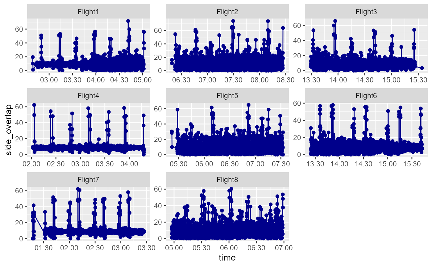

Ground surface resolution in cm/pixel

GSR_all_dfs=dfs_reduced %>% 
  rowwise() %>%mutate("GSD_near"=Kulan::GSD(altitude = alt_above_ground
                                 )[1])%>%  mutate("GSD_mid"=Kulan::GSD(altitude = alt_above_ground)[2]) %>% mutate("GSD_far"=Kulan::GSD(altitude = alt_above_ground)[3])
GSR_all_dfs %>% 
  group_by(Flight) %>% 
  summarise(cm_per_pixel_near=mean(unlist(GSD_near), na.rm=TRUE), sd_cm_per_pixel_near=sd(unlist(GSD_near), na.rm=TRUE),cm_per_pixel_far=mean(unlist(GSD_far), na.rm=TRUE), sd_cm_per_pixel_far=sd(unlist(GSD_far), na.rm=TRUE))

## # A tibble: 8 x 5
##   Flight  cm_per_pixel_near sd_cm_per_pixel_~ cm_per_pixel_far sd_cm_per_pixel_~
##   <chr>               <dbl>             <dbl>            <dbl>             <dbl>
## 1 Flight1              2.96            0.0597             4.82            0.0973
## 2 Flight2              2.98            0.0775             4.86            0.126 
## 3 Flight3              2.84            0.0536             4.62            0.0873
## 4 Flight4              2.90            0.0446             4.73            0.0725
## 5 Flight5              2.91            0.0870             4.73            0.142 
## 6 Flight6              2.78            0.0801             4.53            0.131 
## 7 Flight7              2.95            0.0303             4.81            0.0494
## 8 Flight8              2.80            0.0859             4.56            0.140

Distance covered by each flight in KM

(dist_sum=distance_df %>% 
  group_by(Flight) %>% 
  summarise(Distance=sum(coord_dif, na.rm=TRUE)))

## # A tibble: 8 x 2
##   Flight  Distance
##   <chr>      <dbl>
## 1 Flight1  206258.
## 2 Flight2  189100.
## 3 Flight3  181322.
## 4 Flight4  197963.
## 5 Flight5  189830.
## 6 Flight6  199584.
## 7 Flight7  185306.
## 8 Flight8  165351.

Generate summary ouputs

Flight summary table

dfs_reduced<-dfs_reduced %>% inner_join(.,overlap_all)

## Joining, by = c("photo_no", "alt_above_ground", "banking_angle", "Flight")

dfs_reduced$Rel_for_over <- (dfs_reduced$forward_overlap/dfs_reduced$photo_area_R)*100  # add relative forward overlap

dfs_reduced<-dfs_reduced %>% inner_join(., GSR_all_dfs)

## Joining, by = c("photo_no", "date", "time", "lat_dec", "lon_dec", "alt_above_the_sea_level", "alt_above_launch_point", "alt_above_ground", "banking_angle", "tangage", "azimuth", "gps_course", "speed", "gps_speed", "camera_position", "species", "number", "Flight", "v18", "strip_width", "photo_area_R", "photo_area_L", "side_overlap")

no_photos=dfs_reduced %>% 
  group_by(Flight) %>% 
  tally()

dfs_reduced<-dfs_reduced %>% inner_join(no_photos)

## Joining, by = "Flight"

output_summary_table <- dfs_reduced %>% 
  group_by(Flight) %>% 
  summarise(Date=min(date), Time_start=min(time), Time_end=max(time), 
            Mean_Altitude=mean(alt_above_ground, na.rm=TRUE), #SD_Altitude=sd(alt_above_ground, na.rm=TRUE), 
            Mean_GPS_Speed=mean(gps_speed, na.rm=TRUE), #SD_GPS_Speed=sd(gps_speed, na.rm=TRUE),
            Mean_GPS_dist=mean(coord_dif, na.rm=TRUE), #SD_coord_dif=sd(coord_dif, na.rm=TRUE),
            Mean_Banking= mean(banking_angle, na.rm=TRUE), #SD_Banking=sd(banking_angle, na.rm=TRUE), 
            Mean_Stripw_right=mean(strip_width, na.rm=TRUE), #SD_Stripw_right=sd(strip_width, na.rm=TRUE),
            Mean_GSD_near=mean(unlist(GSD_near), na.rm=TRUE), Mean_GSD_mid=mean(unlist(GSD_mid), na.rm=TRUE), Mean_GSD_far=mean(unlist(GSD_far), na.rm=TRUE),
            Mean_Photo_area_R=mean(photo_area_R, na.rm=TRUE), #SD_Photo_area=sd(photo_area, na.rm=TRUE)
            Mean_Photo_area_L=mean(photo_area_L, na.rm=TRUE),#SD_Photo_area=sd(photo_area, na.rm=TRUE)
            Mean_side_overlap=mean(side_overlap, na.rm=TRUE), #SD_side_overlap=sd(side_overlap, na.rm=TRUE)) 
            Rel_side_overlap=(Mean_side_overlap/Mean_Stripw_right)*100, #% side overlap
            Mean_for_overlap=mean(forward_overlap, na.rm=TRUE), #SD_forward_overlap=sd(forward_overlap, na.rm=TRUE)) 
            Rel_for_overlap=(Mean_for_overlap/Mean_Photo_area_R)*100) #% forward overlap

no_photos <- dfs_reduced %>% 
  group_by(Flight) %>%
  tally()

names(no_photos)[2] <- "N_photos_right"

output_summary_table <- output_summary_table %>% 
                        inner_join(no_photos, by=c("Flight"="Flight"))

output_summary_table %>% view()
# You can write the table to .csv using this code below
#write.csv(output_summary_table, "Summary_per_Flight.csv")

kableExtra::kable(output_summary_table) %>% 
  kableExtra::kable_styling()

Flight	Date	Time_start	Time_end	Mean_Altitude	Mean_GPS_Speed	Mean_GPS_dist	Mean_Banking	Mean_Stripw_right	Mean_GSD_near	Mean_GSD_mid	Mean_GSD_far	Mean_Photo_area_R	Mean_Photo_area_L	Mean_side_overlap	Rel_side_overlap	Mean_for_overlap	Rel_for_overlap	N_photos_right
Flight1	16.07.2020	02:39:02	05:01:43	230.0482	87.30400	123.9532	-0.2970571	307.2174	2.959628	3.783562	4.820468	63150.85	64780.96	10.107387	3.289979	24995.57	39.58073	1665
Flight2	16.07.2020	06:19:00	08:26:52	231.7539	87.74318	126.9129	-0.2454058	316.1448	2.981851	3.811402	4.856385	64820.18	66520.87	11.706242	3.702810	24345.30	37.55821	1491
Flight3	16.07.2020	13:29:24	15:34:09	220.6883	86.57092	128.9628	-0.0968017	297.6395	2.839474	3.629268	4.624449	58595.62	60119.04	9.831595	3.303189	21796.69	37.19849	1407
Flight4	17.07.2020	02:01:37	04:18:01	225.7291	86.85670	120.9305	-0.1415751	300.9421	2.904310	3.712430	4.730134	60911.70	62480.83	9.355282	3.108666	24299.73	39.89337	1638
Flight5	17.07.2020	05:21:48	07:32:28	225.8599	86.89314	126.8068	0.0208945	309.2690	2.905995	3.714393	4.732890	62042.96	63675.35	11.049560	3.572799	22825.89	36.79046	1498
Flight6	17.07.2020	13:24:26	15:42:26	216.2101	87.96046	109.7221	-0.0798901	290.4986	2.781764	3.555775	4.530473	56222.16	57679.71	9.235642	3.179238	23597.91	41.97261	1820
Flight7	18.07.2020	01:17:22	03:26:59	229.6322	83.69114	128.5060	0.0120582	310.6047	2.954615	3.776292	4.811809	63588.06	65243.11	10.075753	3.243915	28379.81	44.63073	1443
Flight8	18.07.2020	04:57:29	06:58:56	217.5620	83.15225	107.9314	-0.1504240	296.2667	2.799185	3.577991	4.558917	57208.30	58707.40	10.570364	3.567854	23426.34	40.94920	1533